From Two Policies to Three: Extending TRPO under Behavior–Reference Policy Mismatch in LLM RL

1. Training–Inference Mismatch and Asynchronous Frameworks

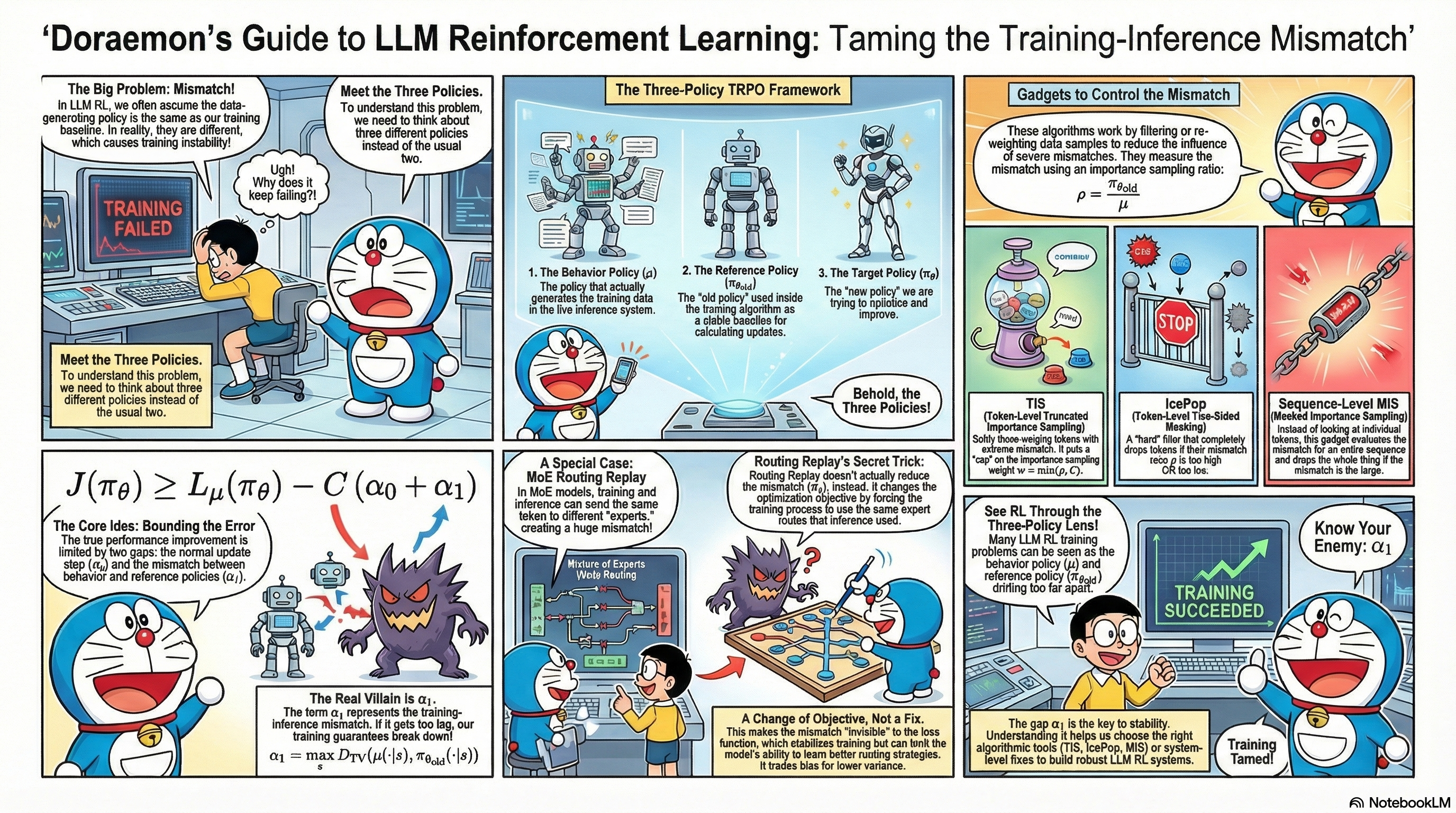
Recent LLM RL work has repeatedly run into the same issue: the behavior policy that actually generates data may not match the reference policy used in training.

This note first reviews the pieces of prior work that matter most for the story, then organizes them around that single mismatch.

I am not trying to prove a stronger TRPO theorem here. What I care about is separating three policies that are often collapsed together in LLM RL, and using that split to say more precisely what training-inference mismatch is actually breaking.

More concretely, this note does only three things:

• rewrites the usual TRPO surrogate gap with the behavior policy as the baseline;
• upper-bounds that gap using behavior, reference, and target policies simultaneously;
• uses that decomposition to reread training-inference mismatch, sample-level correction, and routing replay in LLM RL.

Throughout the note I’ll use:

• Behavior policy $\mu$: the policy that actually generates rollouts, i.e., “under which distribution your data are sampled.” In modern LLM RL systems this typically corresponds to the implementation inside the inference engine (vLLM, SGLang, etc.), and under asynchronous frameworks it is often a mixture distribution over multiple worker policies.

• Reference policy $\pi_{\theta_{\text{old}}}$: the policy used in the training objective for importance sampling, clipping, or KL constraints — typically the “old policy” in PPO / GRPO.

• Target policy $\pi_\theta$: the policy we optimize in the training objective, i.e., “what we want the model to become” — typically the “new policy” in PPO / GRPO.

In the classical idealized setup, we usually implicitly assume $\mu = \pi_{\theta_{\text{old}}}$. In real systems, however, asynchronous updates, different inference / training backends, MoE routing fluctuations, and even hardware-level numerical differences cause these two policies to deviate to varying degrees.

2. Related Work

Below is a selective list of works that matter most for the three-policy story.

• Decoupled PPO was among the first to point out that in trust-region policy optimization methods (TRPO and PPO), the “old policy” actually plays two distinct roles:

  1. It is used for importance sampling to perform off-policy correction. In this sense, the “old policy” is meant to represent the behavior policy that generated the training data.

  2. It is also used to limit the update step size of the new policy. In this sense, the “old policy” acts as a baseline to measure how much the new and old policies differ, i.e., a proximal policy (what I call the reference policy here).

  The paper points out that these two roles do not have to be played by the same policy, and proposes the Decoupled PPO objective, which explicitly decouples “who generates the data” from “who defines the trust region” at the level of the optimization objective.

• AReaL focuses on the mismatch between behavior and reference policies under asynchronous training frameworks: rollouts are often generated by stale parameter versions or different workers. The paper adopts a Decoupled-PPO-style objective in the asynchronous setting, explicitly separating the behavior distribution from the reference policy, while still maintaining PPO-like optimization properties in this asynchronous regime.

• GSPO starts from stability issues of GRPO on long sequences and MoE models. It shows that token-level PPO / GRPO can become highly unstable when MoE expert routing is extremely volatile (especially when routing differs significantly between old and new policies), leading to large variance and training collapse. GSPO proposes a sequence-level PPO-style objective and ratio constraint, using the ratio over entire sequences to control updates. This substantially mitigates training collapse in MoE scenarios caused by routing instability and token-level noise.

• Your Efficient RL Framework Secretly Brings You Off-Policy RL Training observes that in existing LLM RL frameworks (such as VeRL), the inference stack and the training stack often differ across multiple functional modules (e.g., vLLM vs. FSDP / Megatron kernels and operators). This makes the behavior policy $\mu$ differ from the reference policy $\pi_{\theta_{\text{old}}}$, so what is assumed to be on-policy training actually becomes off-policy training with nontrivial bias. The article summarizes two existing ways to handle this: PPO-IS and vanilla-IS, and further proposes token-level truncated importance sampling (TIS) to downweight samples with severe training–inference mismatch. The author also wrote two more foundational notes analyzing training–inference mismatch from basic principles: Part I and Part II.

• Defeating Nondeterminism in LLM Inference points out that the lack of batch-size invariance is a core source of randomness in LLM inference: the same input can yield noticeably different probability distributions under different batch compositions and kernel paths. This means that even when you “nominally” have a single set of parameters, the behavior policy $\mu$ realized in practice can fluctuate with system load and scheduling, further exacerbating training–inference mismatch.

• Small Leak Can Sink a Great Ship—Boost RL Training on MoE with 𝑰𝒄𝒆𝑷𝒐𝒑! observes that the above mismatch issues are further amplified in MoE models: routing itself is highly sensitive to small perturbations, and stacked with inference / training implementation differences and asynchronous sampling, it is easy to magnify bias and instability. The paper proposes IcePop: at the token level, it computes importance sampling ratios and applies two-sided masking to discard tokens whose ratios are either too large or too small. This removes “very noisy” data from the gradient, stabilizing RL training on MoE models.

• When Speed Kills Stability: Demystifying RL Collapse from the Training-Inference Mismatch gives a systematic analysis of the causes of training–inference mismatch, including large amounts of out-of-distribution and low-probability content introduced by agent workflows, hardware and kernel-level numerical uncertainty, and how token-level importance sampling can introduce severe bias on long sequences. It further proposes sequence-level masked importance sampling (sequence-level MIS): compute an IS ratio at the sequence level and discard only those sequences whose overall ratio is too large, thereby controlling bias while strongly suppressing training collapse caused by extreme samples. The paper provides reasonably complete theoretical derivations and extensive experimental evidence.

• Stabilizing MoE Reinforcement Learning by Aligning Training and Inference Routers focuses on the MoE-specific problem of routing inconsistency. The paper finds that even for identical inputs, inference and training can route tokens to different experts due to small differences in operator implementations or parallelism. This “physical-path” mismatch makes the gap between the behavior policy $\mu$ and the reference policy $\pi_{\theta_{\text{old}}}$ much larger than expected and can easily cause training collapse. To address this, the paper proposes Rollout Routing Replay (R3): during rollout it records, for each token, the actual expert indices selected by the inference router, and during training it replays these routing decisions instead of recomputing them. In effect, R3 forces the training and inference stacks to share the same routing paths in the MoE topology, aligning the two sides at the level of the computation graph.

• RL 老训崩？训推差异是基石 approaches the problem more from a practical perspective, sharing experience on how to engineer for near training–inference consistency: choosing consistent operators and precision settings, monitoring and constraining the log-prob gap between training and inference, etc. The focus is on framework-level engineering practices that can mitigate training–inference difference at the root.

• verl Rollout Importance Sampling introduces a Token Veto mechanism in its rollout correction module: it computes token-level importance ratios $\rho_t^{(\text{ref}\leftarrow\text{beh})}$, and if any token in a trajectory satisfies $\min_t \rho_t < \tau_{\text{veto}}$, the entire sequence is discarded from training. This “token-level detection, sequence-level veto” design embodies a conservative “one-vote veto” strategy.

• INTELLECT-3 Technical Report adopts a similar rejection sampling strategy in its asynchronous distributed RL training framework. INTELLECT-3 computes token-level importance ratios for each rollout; if any token’s ratio falls below a threshold ($10^{-5}$ in the paper), the entire trajectory is masked.

3. Three-Policy TRPO: A Minimal Unifying Frame

At first glance, the works listed above seem to tackle different aspects:

• Algorithmic level: how to formulate PPO / GRPO objectives, token-level vs. sequence-level, clip vs. mask, etc.
• Systems level: how to align inference and training stacks.
• Model level: how MoE routing amplifies instability, and so on.

However, if we organize everything along a single axis — behavior policy vs. reference policy — most of these issues fit inside one minimal frame: three-policy TRPO.

The derivation is short. First write the surrogate gap with the behavior policy as baseline; then add one triangle inequality and the two mismatch sources appear. What surprised me is how useful this tiny split is once you start looking at modern LLM RL systems through it:

• On the one hand, it helps us understand what exactly “training–inference mismatch” and “asynchronous training frameworks” are harming within the TRPO view.
• On the other hand, it offers a unifying way to interpret TIS, IcePop, sequence-level MIS, etc. In the view of this note, these methods mostly mitigate the estimation bias/variance consequences of behavior-reference mismatch, rather than directly changing the worst-case value of $\alpha_1$.

3.1 Three Policies

We stick to the notation from above and consider a discounted MDP with discount factor $\gamma \in (0,1)$:

For LLM RL, many workloads are closer to finite-horizon sequence decision problems than to infinite-horizon discounted MDPs. I still use the discounted-MDP notation here because it connects most directly to the classical TRPO derivation; the same decomposition carries over to finite-horizon versions as well.

• States $s \in \mathcal{S}$, actions $a \in \mathcal{A}$.
• Policy $\pi(a \mid s)$.
• Discounted state distribution: $$ d_\pi(s) := (1-\gamma)\sum_{t=0}^\infty \gamma^t \Pr_\pi(s_t = s). $$
• Return (episodic view): $$ \mathcal{J}(\pi) := \mathbb{E}_\pi\Big[\sum_{t=0}^\infty \gamma^t r_t\Big]. $$
• Value / Q / advantage functions: $$ V_\pi(s),\quad Q_\pi(s,a),\quad A_\pi(s,a) := Q_\pi(s,a) - V_\pi(s). $$

I keep the notation from the introduction: behavior policy $\mu$, reference policy $\pi_{\theta_{\text{old}}}$, and target policy $\pi_\theta$.

In the ideal setup we assume $\mu = \pi_{\theta_{\text{old}}}$; in real systems they are often unequal. This is the mathematical shadow of “training–inference mismatch.”

3.2 Two-Policy TRPO: A Behavior-Baselined Surrogate-Gap Bound

If you’re already familiar with TRPO, feel free to skip ahead to the “Three-Policy TRPO” subsection.

I keep the core TRPO logic, but I will not try to reproduce the exact theorem statement from Schulman et al. (2015). For the three-policy story below, a looser behavior-baselined surrogate-gap bound is the more useful object.

All the theoretical guarantees in TRPO are stated with respect to the advantage function of some baseline policy. Here I take $\mu$ as the baseline for two reasons: the data are sampled under $\mu$, and in practice the critic / GAE / group-normalized reward proxy we can estimate most naturally from those data is also anchored to that behavior distribution. I ignore the approximation error in estimating $A_\mu$ itself and focus only on the policy-mismatch part.

A classical result is the Performance Difference Lemma:

For any two policies $\mu$ and $\pi_\theta$, we have

$$ \mathcal{J}(\pi_\theta) - \mathcal{J}(\mu) = \frac{1}{1-\gamma}\; \mathbb{E}_{s\sim d_{\pi_\theta},\, a\sim\pi_\theta}[A_\mu(s,a)]. $$

The challenge in TRPO is that we cannot compute

$$ \mathbb{E}_{s\sim d_{\pi_\theta}, a\sim\pi_\theta}[A_\mu(s,a)] $$

exactly, because $d_{\pi_\theta}$ is the state distribution of the new policy, under which we do not have samples.

So TRPO introduces a surrogate objective by replacing the state distribution with that of the behavior policy:

$$ L_\mu(\pi_\theta) := \mathcal{J}(\mu) + \frac{1}{1-\gamma}\mathbb{E}_{s\sim d_\mu,\,a\sim \pi_\theta}[A_\mu(s,a)]. $$

In actual PPO / GRPO-style implementations, this expectation is usually rewritten using importance sampling. That is also where a second policy often enters the picture: the denominator in the ratio is frequently the reference policy $\pi_{\theta_{\text{old}}}$ rather than the true behavior policy $\mu$. The gap between those two is exactly what will become $\alpha_1$ later.

Starting from the Performance Difference Lemma, the difference between the true objective and the surrogate is:

$$ \mathcal{J}(\pi_\theta) - L_\mu(\pi_\theta) = \frac{1}{1-\gamma}\; \sum_s \big(d_{\pi_\theta}(s) - d_\mu(s)\big) \,\mathbb{E}_{a\sim\pi_\theta(\cdot\mid s)}[A_\mu(s,a)]. $$

If we define

$$ \epsilon_\mu := \max_{s,a} |A_\mu(s,a)|, $$

we immediately get the following upper bound:

Lemma 1

$$ |\mathcal{J}(\pi_\theta) - L_\mu(\pi_\theta)| \le \frac{\epsilon_\mu}{1-\gamma}\; \|d_{\pi_\theta} - d_\mu\|_1. $$

This reveals the first key quantity:

State distribution shift $\|d_{\pi_\theta} - d_\mu\|_1$, i.e., “how differently the new policy sees the world, compared to the behavior policy.”

We usually do not directly impose constraints on $\|d_{\pi_\theta} - d_\mu\|_1$. Instead, we constrain the per-timestep action distribution difference — via trust regions, KL penalties, clipping, etc.

Define the total variation (TV) distance:

$$ D_{\mathrm{TV}}(p,q) := \frac{1}{2}\|p-q\|_1. $$

Assume there is a constant $\beta$ such that

For all $s$, the TV distance between the behavior and target policies is bounded:

$$ D_{\mathrm{TV}}\big(\mu(\cdot\mid s), \pi_\theta(\cdot\mid s)\big) \le \beta. $$

Intuitively: in any state, the action distribution of the “new policy” cannot deviate too much from that of the policy that generated the data.

A standard result (provable via coupling) is:

Lemma 2 Under the assumption above,

$$ \|d_{\pi_\theta} - d_\mu\|_1 \le \frac{2\gamma}{1-\gamma}\,\beta. $$

Combining Lemma 1 and Lemma 2, we obtain

$$ |\mathcal{J}(\pi_\theta) - L_\mu(\pi_\theta)| \le \frac{\epsilon_\mu}{1-\gamma}\; \frac{2\gamma}{1-\gamma}\,\beta = \frac{2\epsilon_\mu\gamma}{(1-\gamma)^2}\,\beta. $$

This gives a compact two-policy surrogate-gap bound with the behavior policy as baseline:

Theorem 1 (Behavior-Baselined Two-Policy Bound)

$$ \mathcal{J}(\pi_\theta) \;\ge\; L_\mu(\pi_\theta) \;-\; \frac{2\epsilon_\mu\gamma}{(1-\gamma)^2}\,\beta. $$

This suggests:

• What really matters for the tightness of $L_\mu(\pi_\theta)$ as a surrogate for $\mathcal{J}(\pi_\theta)$ is how far the behavior policy $\mu$ and the target policy $\pi_\theta$ drift apart: $$ \beta = \max_s D_{\mathrm{TV}}\big(\mu(\cdot\mid s), \pi_\theta(\cdot\mid s)\big). $$

If you can directly control this $\beta$, you can essentially port TRPO’s monotonic-improvement logic to the behavior-policy view. This is a deliberately conservative worst-case-TV presentation: the goal here is to make the structure transparent, not to optimize constants. If you switch to an average-TV version, you get a similar conclusion closer to sample averages, with modified constants and expectations.

3.3 Three-Policy TRPO

In practice, especially in large-scale LLM RL, we often cannot directly control $\beta$ itself.

In most PPO / GRPO / GSPO / RLHF-style frameworks, the actual situation is:

• Rollout data are generated by some behavior policy $\mu$ (some particular parameter version plus system details inside the inference engine).
• During updates, we would like to leverage a reference policy $\pi_{\theta_{\text{old}}}$ to limit the update of the target policy $\pi_\theta$.

Practically, the quantities we can directly control or indirectly influence are:

1. Reference vs. target: via KL penalties, clipping, etc., we constrain

   $$ D_{\mathrm{TV}}\big(\pi_{\theta_{\text{old}}}(\cdot\mid s),\pi_\theta(\cdot\mid s)\big). $$

2. Behavior vs. reference: we would like to keep $$ D_{\mathrm{TV}}\big(\mu(\cdot\mid s),\pi_{\theta_{\text{old}}}(\cdot\mid s)\big) $$ small as well — this is where training–inference mismatch and asynchronous execution come in.

This motivates two deviation sources, corresponding to two TV-distance terms:

• Deviation source A: reference vs. target

  $$ \alpha_0 := \max_s D_{\mathrm{TV}}\big(\pi_{\theta_{\text{old}}}(\cdot\mid s), \pi_\theta(\cdot\mid s)\big); $$

• Deviation source B: behavior vs. reference $$ \alpha_1 := \max_s D_{\mathrm{TV}}\big(\mu(\cdot\mid s), \pi_{\theta_{\text{old}}}(\cdot\mid s)\big). $$

Intuitively:

• $\alpha_0$: how far the new policy is from the reference policy chosen in the loss — this is the trust-region part.
• $\alpha_1$: how far the reference policy used in training is from the actual behavior policy that generated the data — this is the footprint of training–inference mismatch and asynchrony.

Now we can plug these two quantities back into the TRPO lower bound.

For any state $s$, by the triangle inequality we have

$$ \begin{aligned} D_{\mathrm{TV}}\big(\mu(\cdot\mid s),\pi_\theta(\cdot\mid s)\big) &\le D_{\mathrm{TV}}\big(\mu(\cdot\mid s),\pi_{\theta_{\text{old}}}(\cdot\mid s)\big) \\ &\quad + D_{\mathrm{TV}}\big(\pi_{\theta_{\text{old}}}(\cdot\mid s),\pi_\theta(\cdot\mid s)\big). \end{aligned} $$

Taking the supremum over $s$ gives

$$ \beta := \max_s D_{\mathrm{TV}}\big(\mu(\cdot\mid s),\pi_\theta(\cdot\mid s)\big) \;\le\; \alpha_1 + \alpha_0. $$

Plugging this inequality into the two-policy TRPO bound (Theorem 1), and denoting

$$ C := \frac{2\epsilon_\mu\gamma}{(1-\gamma)^2}, $$

we obtain

$$ \mathcal{J}(\pi_\theta) \;\ge\; L_\mu(\pi_\theta) \;-\; C\,\beta \;\ge\; L_\mu(\pi_\theta) \;-\; C\,(\alpha_0 + \alpha_1). $$

This yields a very direct three-policy TRPO lower bound:

Theorem 2 (Three-Policy TRPO) Let

$$ \epsilon_\mu := \max_{s,a} |A_\mu(s,a)|,\quad C := \frac{2\epsilon_\mu\gamma}{(1-\gamma)^2}, $$

and

$$ \alpha_0 := \max_s D_{\mathrm{TV}}\big(\pi_{\theta_{\text{old}}}(\cdot\mid s), \pi_\theta(\cdot\mid s)\big), \quad \alpha_1 := \max_s D_{\mathrm{TV}}\big(\mu(\cdot\mid s), \pi_{\theta_{\text{old}}}(\cdot\mid s)\big). $$

Then for any target policy $\pi_\theta$,

$$ \boxed{ \mathcal{J}(\pi_\theta) \;\ge\; L_\mu(\pi_\theta) \;-\; C\,(\alpha_0 + \alpha_1) } $$

where

$$ L_\mu(\pi_\theta) := \mathcal{J}(\mu) + \frac{1}{1-\gamma} \mathbb{E}_{s\sim d_\mu,a\sim\pi_\theta}[A_\mu(s,a)]. $$

The point of Theorem 2 is simple: the gap between $L_\mu(\pi_\theta)$ and $\mathcal{J}(\pi_\theta)$ is not exactly decomposed into two terms, but it is controlled by a conservative upper bound involving both $\alpha_0$ and $\alpha_1$. To get improvement you still need $L_\mu(\pi_\theta)$ itself to be large enough. Numerically this bound is often loose in LLM settings, so I read it mainly as a structural tool rather than a performance certificate.

3.4 How to Control These Two Deviation Sources?

We can now revisit various practical methods through the lens of Theorem 2:

• Most PPO / GRPO-style work focuses on the reference-vs.-target side, i.e. $\alpha_0$.
• GSPO belongs to the same side, but it does something stronger than “control $\alpha_0$ more carefully”: it changes the basic unit of ratio, clipping, and optimization from token level to sequence level.
• TIS / IcePop / MIS / WTRS mostly operate on sample weights, sample subsets, or rejection rules to mitigate the estimation consequences of behavior-vs.-reference mismatch, rather than directly changing the worst-case definition of $\alpha_1$.

If I had to say which side worries me more in practice, it is almost always the latter: many systems drift out of the “approximately on-policy” regime because behavior and reference policies have already diverged before the trust-region machinery itself visibly fails. In the remainder of this note I focus on the behavior-vs.-reference side.

The goal on this side is simple: make the effective training data come from a behavior policy close enough to the reference policy, or at least prevent badly mismatched samples from dominating the gradient.

In practice, this usually involves both system-level mechanisms and algorithmic mechanisms (importance sampling).

1. System level: keep behavior and reference policies close

   • Asynchronous frameworks: Tag each sample with a policy version, and only use data generated by parameter versions that are close enough to $\pi_{\theta_{\text{old}}}$.

   • Training–inference alignment: Use consistent precision, operators, and similar kernel behavior between the training and inference stacks.

   These mechanisms act “outside” the algorithm to make $\mu$ closer to $\pi_{\theta_{\text{old}}}$, thereby reducing $\alpha_1$ more directly.

2. Algorithmic level: sample-wise correction

   At the algorithmic level, we no longer attempt to “fix” the entire behavior policy. Instead, we use importance sampling ratios to filter or reweight samples at the sample level, so that the subset of data that actually participates in training is closer to the reference policy, or at least so that badly mismatched samples carry less weight.

   Concretely, this gives rise to methods like TIS, IcePop, MIS, and WTRS. They are best understood as different ways to manage the consequences of this mismatch at training time.

4. Importance Sampling and Masking: Four Sample-Level Responses to Behavior-Reference Mismatch

In this section I reuse the notation above to write down four representative mechanisms, focusing only on the design choices related to “behavior vs. reference policy.” The unified notation below is meant to highlight how this mismatch is handled in the training loss, not to reproduce every implementation detail from each paper (advantage estimation, baselines, extra regularizers, and so on). The losses $L_{\text{TIS}}, L_{\text{IcePop}}, L_{\text{MIS}}, L_{\text{WTRS}}$ are therefore comparison devices, not literal unbiased estimators of the theoretical surrogate $L_\mu$. Let the token-level PPO / GRPO-style update term be

$$ g_\theta(t) = \min\big(r_t(\theta) A_t,\ \text{clip}(r_t(\theta),1-\epsilon,1+\epsilon) A_t\big), $$

where

$$ r_t(\theta) = \frac{\pi_\theta(a_t\mid s_t)}{\pi_{\theta_{\text{old}}}(a_t\mid s_t)}, \quad (s_t,a_t)\sim\mu. $$

Here:

• $r_t(\theta)$ is the target-vs.-reference ratio.
• $A_t$ denotes the practical advantage term corresponding to the theoretical $A_\mu(s_t,a_t)$. In real implementations it typically comes from a critic / GAE / group-normalized reward proxy estimated from $\mu$-sampled data, so it should not be read as a literal unbiased replacement for $A_\mu$.

To connect token-level $(s_t,a_t)$ with sequence-level $(x,y)$ notation, consider the RLHF setting (reinforcement learning from human feedback) for LLMs:

• Prompts are denoted by $x$, and responses by $y = (y_1,\dots,y_{|y|})$.
• Token-level states and actions are defined as $s_t := (x,y_{
• The behavior and reference policies on sequences can then be written as $$ \mu(y\mid x) = \prod_{t=1}^{|y|}\mu(a_t=y_t\mid s_t),\quad \pi_{\theta_{\text{old}}}(y\mid x) = \prod_{t=1}^{|y|}\pi_{\theta_{\text{old}}}(a_t=y_t\mid s_t). $$

To quantify the deviation between reference and behavior policies, we can define the token-level importance ratio:

$$ \rho_t^{(\text{ref}\leftarrow\text{beh})} := \frac{\pi_{\theta_{\text{old}}}(a_t\mid s_t)}{\mu(a_t\mid s_t)}, $$

and its sequence-level counterpart:

$$ \rho(y\mid x) := \frac{\pi_{\theta_{\text{old}}}(y\mid x)}{\mu(y\mid x)} = \prod_{t=1}^{|y|} \rho_t^{(\text{ref}\leftarrow\text{beh})}. $$

The difference between TIS, IcePop, and MIS lies in how they use $\rho$ to manage behavior-reference mismatch during training.

4.1 TIS: Token-Level Truncated Importance Sampling

TIS directly truncates the token-level ratio $\rho_t^{(\text{ref}\leftarrow\text{beh})}$; define

$$ \color{blue}{w_t = \min\big(\rho_t^{(\text{ref}\leftarrow\text{beh})},\ C_{\text{IS}}\big)}. $$

The update objective becomes

$$ L_{\text{TIS}}(\theta) = - \mathbb{E}_{(s_t,a_t)\sim\mu}\big[\,\color{blue}{w_t}\; g_\theta(t)\big]. $$

• The blue $\color{blue}{w_t}$ is the truncated IS weight: extremely large ratios are capped at a constant $C_{\text{IS}}$.
• From the three-policy TRPO perspective, this is a soft way to downweight tokens where behavior and reference policies differ significantly, thereby reducing their influence on the effective training distribution.
• Note that $w_t$ truncates the behavior-to-reference ratio, while the clipping inside $g_\theta(t)$ controls the reference-to-target ratio. These are two separate operations.

4.2 IcePop: Token-Level Two-Sided Masking in MoE

IcePop also uses $\rho_t^{(\text{ref}\leftarrow\text{beh})}$ as a discrepancy measure, but opts for two-sided masking:

$$ \color{blue}{m_t = \mathbf{1}\big[C_{\text{low}} \le \rho_t^{(\text{ref}\leftarrow\text{beh})} \le C_{\text{high}}\big]}. $$

The update objective becomes

$$ L_{\text{IcePop}}(\theta) = - \mathbb{E}_{(s_t,a_t)\sim\mu}\big[\,\color{blue}{m_t}\; g_\theta(t)\big]. $$

• The blue $\color{blue}{m_t}$ decides whether a token participates in the update: tokens with ratios that are too large or too small are dropped entirely.
• This is a hard sample selection scheme: only tokens where behavior and reference policies are reasonably aligned (ratios within $[C_{\text{low}}, C_{\text{high}}]$) are kept.

4.3 Sequence-Level MIS: Masked Importance Sampling Over Entire Sequences

The core operation in sequence-level MIS is to retain only sequences whose sequence-level IS ratio is below a threshold $C$, zeroing out the loss for all other sequences:

$$ \color{blue}{ \rho(y\mid x) \leftarrow \rho(y\mid x)\,\mathbf{1}\{\rho(y\mid x)\le C\} } $$

In a unified loss form, this can be written as

$$ L_{\text{MIS}}(\theta) =-\,\mathbb{E}_{(x,y)\sim\mu} \Big[ \color{blue}{\rho(y\mid x)\,\mathbf{1}\{\rho(y\mid x)\le C\}} \;\cdot\; \sum_{t=1}^{|y|}g_\theta(t) \Big]. $$

From the three-policy TRPO viewpoint, sequence-level MIS no longer truncates at the token level. Instead, it performs trajectory-level filtering: it drops trajectories where behavior and reference policies diverge too much, and only optimizes on the subset with $\rho(y\mid x)\le C$. My own bias is that once sequences get long, this sequence-level treatment is usually more honest than token-level patching, because token-level weights get dominated by extremes too easily.

Note: In this unified form, $\rho(y\mid x)$ handles the sequence-level correction from behavior to reference, while $g_\theta(t)$ still handles the token-level update from reference to target. In practice, implementations often add extra truncation or stabilization on top of this basic structure.

4.4 A Veto-Style Extreme: What I Call WTRS

The verl Token Veto mechanism and INTELLECT-3 both use a veto-style rejection idea. For the sake of analysis, I will refer to this shared pattern as Worst Token Reject Sampling (WTRS). This is my umbrella term, not a standard name from either source paper, and the concrete implementations are not identical.

Under that abstraction:

• verl Token Veto: In its rollout correction module, if any token in a trajectory has $\min_t \rho_t < \tau_{\text{veto}}$, the entire sequence is discarded via response_mask. The threshold $\tau_{\text{veto}}$ is user-configurable.

• INTELLECT-3 Token Masking: In its asynchronous distributed RL framework, if any token’s ratio is below $10^{-5}$, the entire trajectory is masked.

The core operation is identical: if any token in a trajectory has an IS ratio below a threshold $\tau$, the entire sequence is rejected from training. This can be written as:

$$ \color{blue}{ m(y\mid x) = \mathbf{1}\Big\{\min_{t=1}^{|y|} \rho_t^{(\text{ref}\leftarrow\text{beh})} \ge \tau\Big\} } $$

In a unified loss form:

$$ L_{\text{WTRS}}(\theta) =-\,\mathbb{E}_{(x,y)\sim\mu} \Big[ \color{blue}{m(y\mid x)} \;\cdot\; \sum_{t=1}^{|y|}g_\theta(t) \Big]. $$

From the three-policy TRPO perspective, WTRS adopts a hybrid “token-level detection, sequence-level veto” strategy: it detects extreme mismatch signals at the token level, and once detected, rejects at the sequence level. This is aggressively conservative. The price is poor sample efficiency; the benefit is that under severe system noise it can be more stable than trying to rescue bad trajectories token by token.

5. MoE Routing Replay: What Does It Actually Do in Three-Policy TRPO?

In MoE (Mixture-of-Experts) models, training–inference mismatch often first appears as routing inconsistency: even with identical parameters, the inference and training stacks may route tokens to different experts because of small differences in operators, parallelism, or numerics. A natural engineering response is routing replay: during rollout (inference), record the actual expert paths, and during training, force the model to reuse these routing decisions.

Modeling assumption: in this section I treat routing choice $z$ as part of the action space, i.e. “choose an expert” and “generate a token” are modeled as a joint decision. Everything below about routing replay as an objective rewrite is conditional on that modeling choice.

These methods are often described as “implementing behavior-reference correction” or even “shrinking $\alpha_1$.” From the three-policy TRPO perspective, a more precise statement is:

Routing replay does not directly shrink the original policy-distance terms; instead, it rewrites the surrogate objective into one that is conditioned on / replaces the routing. It makes routing mismatch invisible in the loss, but it does not actually shrink the true policy distances $\alpha_0$ or $\alpha_1$.

Below I’ll sketch a minimal abstraction that is sufficient to make this concrete.

5.1 Surrogate Objective in MoE: Separating Routing and Token Generation

Abstract an MoE model as a two-stage stochastic decision: “first choose an expert $z$, then generate token $a$ conditioned on that expert.” The target policy can be factorized as

$$ \pi_\theta(a,z\mid s)=\omega_\theta(z\mid s)\,\pi_\theta(a\mid s,z), $$

where:

• $\omega_\theta(z\mid s)$ is the router distribution.
• $\pi_\theta(a\mid s,z)$ is the token distribution conditioned on expert $z$.

In the three-policy TRPO setting, the surrogate objective we actually want to optimize can be written as

$$ L_\mu(\pi_\theta) = \mathcal{J}(\mu) + \frac{1}{1-\gamma} \mathbb{E}_{s\sim d_\mu} \bigg[ \sum_z \omega_\theta(z\mid s)\,F_\theta(s,z) \bigg], $$

where I use

$$ F_\theta(s,z) := \sum_a \pi_\theta(a\mid s,z)\,A_\mu(s,a,z) $$

to denote the expert-level aggregation of advantages.

Here $A_\mu(s,a,z)$ denotes the advantage when “choosing expert $z$ and then generating token $a$” is treated as a joint decision. This section therefore works with an extended model in which routing is made explicit inside the decision process.

The key point is that in the original $L_\mu(\pi_\theta)$, the routing distribution is precisely the current router $\omega_\theta$ that we are updating. RL on MoE is therefore updating not only the token-generation distribution but also the router itself.

5.2 Replaying Behavior-Policy Routing (Behavior-Router Replay / R3-Style)

R3-style methods record, during rollout, the set of experts $M_\mu(s)$ actually selected by the behavior policy on the inference side, and during training force the current policy to route only within this set. This can be written as a “conditional projection” of the routing distribution:

$$ \omega_\theta^{\text{R3}}(z\mid s) := \frac{\omega_\theta(z\mid s)\,\mathbf{1}\{z\in M_\mu(s)\}} {\sum_{z'\in M_\mu(s)}\omega_\theta(z'\mid s)} . $$

The surrogate objective that is actually optimized during training becomes

$$ L_\mu^{\text{R3}}(\pi_\theta) = \mathcal{J}(\mu) + \frac{1}{1-\gamma} \mathbb{E}_{s\sim d_\mu} \bigg[ \sum_{z\in M_\mu(s)} \omega_\theta^{\text{R3}}(z\mid s)\,F_\theta(s,z) \bigg]. $$

Compared to the original $L_\mu(\pi_\theta)$, R3 does not push $\omega_\theta$ closer to $\omega_{\text{old}}$ or $\omega_\mu$. Instead, it:

• replaces the expectation over $z\sim\omega_\theta$ by a conditional expectation over $z\sim\omega_\theta(\cdot\mid z\in M_\mu(s))$, and
• equivalently, shrinks the feasible routing support to $M_\mu(s)$.

So R3 is optimizing a “behavior-routing-conditioned surrogate objective,” rather than the original $L_\mu(\pi_\theta)$. The benefit is substantially reduced variance and improved stability; the cost is that the router’s exploration and update freedom is constrained at every state.

5.3 Replaying Reference-Policy Routing (Reference-Router Replay)

Another class of routing-replay schemes instead reuses the reference policy’s router $\omega_{\text{old}}$. This is equivalent to training a hybrid policy

$$ \hat\pi_\theta(a,z\mid s) := \omega_{\text{old}}(z\mid s)\,\pi_\theta(a\mid s,z), $$

with surrogate objective

$$ L_\mu^{\text{ref-replay}}(\pi_\theta) = \mathcal{J}(\mu) + \frac{1}{1-\gamma} \mathbb{E}_{s\sim d_\mu} \bigg[ \sum_z \omega_{\text{old}}(z\mid s)\,F_\theta(s,z) \bigg]. $$

This has the effect that:

• In the surrogate objective, the router is frozen to the old router $\omega_{\text{old}}$, so the “reference vs. target” discrepancy in routing is simply removed from the loss.
• Training becomes insensitive to how far the new router $\omega_\theta$ drifts from $\omega_{\text{old}}$, thereby sidestepping the instabilities caused by routing mismatch.

Again, this is fundamentally a change of objective:

• The deviation $\alpha_0$ in the true policy space is not reduced; it is merely rendered invisible by redefining the surrogate in terms of the old router.
• Learning of the router is effectively frozen or heavily suppressed.

5.4 Routing Replay as a Change of Surrogate Objective

Putting these replay variants side by side, they share several properties:

1. They optimize not the original $L_\mu(\pi_\theta)$, but a surrogate where routing has been conditioned or replaced.
2. They do not directly shrink the three-policy TRPO bound’s $\alpha_0$ or $\alpha_1$. Routing mismatch is removed from the loss, but it still exists in the true policy distances.
3. In practice they trade bias for variance: replay typically lowers variance and improves stability, but may also limit the router’s ability to learn routing patterns that are optimal for the RL objective.

So, in the three-policy TRPO view, a more accurate characterization is:

Routing replay is best thought of as a rewrite of the surrogate objective, not as a direct implementation of a constraint on $\alpha_0$ or $\alpha_1$.

Put more bluntly: routing replay is often an effective workaround, not a theoretical fix.

6. Discussion

The core claim of this note is:

Many issues around training-inference mismatch and asynchronous training in large-scale LLM RL are easier to understand once you stop collapsing behavior policy and reference policy into the same object; in practice, the missing term is often $\alpha_1$.

From two policies to three, the actual move is small:

• We rewrote the TRPO lower bound from an “old vs. new policy” narrative into a “behavior–reference–target” three-policy relationship.

• We explicitly separated two TV distances:
  • reference vs. target, $\alpha_0$, corresponding to the KL / clip / trust-region style controls in PPO / GRPO / GSPO;
  • behavior vs. reference, $\alpha_1$, capturing real-world factors like asynchronous frameworks, training-inference mismatch, MoE routing volatility, kernel-level nondeterminism, etc.
• This leads to a simple conclusion: The gap between the surrogate $L_\mu(\pi_\theta)$ and the true performance $\mathcal{J}(\pi_\theta)$ is bounded by $C(\alpha_0 + \alpha_1)$.

Under this lens:

• Decoupled PPO / AReaL can be viewed as formally acknowledging the existence of three policies and explicitly decoupling the behavior distribution from the reference policy in the objective.

• PPO / GRPO primarily control the reference-vs.-target side; GSPO also lives on that side, but it does so by changing the optimization unit from token level to sequence level.
• TIS, IcePop, MIS, and WTRS can be seen as different ways of managing the training-time consequences of behavior-reference mismatch:
  • TIS: token-level truncation of IS weights to soften the influence of extreme samples.
  • IcePop: token-level two-sided masking in MoE to hard-drop tokens with severe mismatch.
  • MIS: sequence-level masking to ignore entire trajectories whose behavior–reference mismatch is too large.
  • WTRS: token-level detection of extremely small ratios, rejecting the entire trajectory once such a signal is found.

• Routing replay (whether replaying behavior routing in R3-style schemes or replaying reference routing) is better viewed as changing the surrogate objective rather than directly implementing a constraint: both variants replace the original $L_\mu(\pi_\theta)$ with a routing-conditioned / routing-frozen surrogate, trading off some objective bias and reduced routing learning freedom for lower variance and greater stability, without actually shrinking $\alpha_0$ or $\alpha_1$—they simply make routing mismatch invisible in the loss.

• Engineering advice such as in RL 老训崩？训推差异是基石 and system-level work like Defeating Nondeterminism in LLM Inference can be interpreted as efforts to reduce $\alpha_1$ on the systems and numerical side, so that the assumptions underlying the algorithms do not break too badly.

One more practical point matters here: Theorem 2 is written in terms of worst-case TV distances, which are almost impossible to observe directly in LLM-scale systems. What you can usually monitor instead are engineering proxies: average KL on logged states, quantiles of token- or sequence-level importance weights, effective sample size (ESS), rejection / masking rate, and staleness across asynchronous workers. The theorem tells you which mismatches matter; the proxies tell you when they are getting out of hand.

If I had to pick one side to watch first in a real system, it would usually be $\alpha_1$. That side is easier to ignore, and in practice it often breaks the “approximately PPO / TRPO” regime before the nominal trust-region machinery does.

From this perspective, two practical questions seem especially worth chasing:

• Under what conditions can we still reasonably interpret “LLM RL training” as some approximate form of TRPO / PPO?
• For a concrete RL system, should we spend effort first on tighter $\alpha_0$ control or on pushing $\alpha_1$ back into a tolerable regime? My bias is the latter: once the behavior distribution has drifted too far, a beautiful trust region is constraining the wrong object.

If this note is useful at all, I hope it is because it makes one neglected point harder to ignore: many things that look like “PPO instability” are already broken one step earlier, at $\mu \neq \pi_{\theta_{\text{old}}}$. Writing the three policies separately is often the fastest way to see where the real bottleneck sits.

References

1. John Schulman, Sergey Levine, Philipp Moritz, Michael I. Jordan, Pieter Abbeel. “Trust Region Policy Optimization” (TRPO). arXiv:1502.05477. https://arxiv.org/abs/1502.05477
2. Jacob Hilton, Karl Cobbe, John Schulman. “Batch size-invariance for policy optimization” (Decoupled PPO). arXiv:2110.00641. https://arxiv.org/abs/2110.00641
3. Joshua Achiam, David Held, Aviv Tamar, Pieter Abbeel. “Constrained Policy Optimization” (CPO). arXiv:1705.10528. https://arxiv.org/abs/1705.10528
4. James Queeney, Ioannis Ch. Paschalidis, Christos G. Cassandras. “Generalized Proximal Policy Optimization with Sample Reuse” (GePPO). arXiv:2111.00072. https://arxiv.org/abs/2111.00072
5. Wei Fu, Jiaxuan Gao, Xujie Shen, et al. “AReaL: A Large-Scale Asynchronous Reinforcement Learning System for Language Reasoning”. arXiv:2505.24298. https://arxiv.org/abs/2505.24298
6. Chujie Zheng, Shixuan Liu, Mingze Li, et al. “Group Sequence Policy Optimization” (GSPO). arXiv:2507.18071. https://arxiv.org/abs/2507.18071
7. Wenhan Ma, Hailin Zhang, Liang Zhao, et al. “Stabilizing MoE Reinforcement Learning by Aligning Training and Inference Routers”. arXiv:2510.11370. https://arxiv.org/abs/2510.11370

@misc{WangZhang2025ThreePolicyTRPO,
  author       = {Wang, Xihuai and Zhang, Shao},
  title        = {From Two Policies to Three: Extending TRPO under Behavior-Reference Policy Mismatch in LLM RL},
  year         = {2025},
  month        = nov,
  day          = {15},
  url          = {https://xihuai18.github.io/reinforcement-learning/2025/11/15/three-policy-en.html},
  urldate      = {2025-11-23}
}