Choosing KL Estimators in RL: From Value Unbiasedness to Gradient Correctness

In RL, KL estimators should not be judged only by how accurately they estimate KL values, but also by what objective their gradients actually optimize. This post compares three estimators $k_1, k_2, k_3$ in both on-policy and off-policy settings, and shows how the answer changes depending on whether KL is used as a differentiable loss term or as a detached reward-shaping term.

1. Introduction: The Role of KL Divergence in Reinforcement Learning

This post is really about one implementation-level question: when code says “add a KL penalty,” why can changing the estimator, changing the sampling distribution, or adding a single .detach() quietly change the optimization target? In policy optimization (PPO, GRPO, etc.) and alignment training (RLHF/RLAIF), a KL penalty looks like a straightforward regularizer that keeps the current policy close to a reference. But once you implement it, several choices immediately branch apart: which estimator ($k_1$, $k_2$, $k_3$), which sampling distribution (on-policy vs. off-policy), and how the KL term enters optimization (as a differentiable loss term vs. as a detached reward-shaping term).

To make that question precise, we need to separate two issues: estimating the value of a KL term, and understanding which objective its gradient actually optimizes. In many implementations those are not the same thing.

1.1 The Distinction Between Forward KL and Reverse KL

Let $q_\theta$ be the current actor policy, $p$ the reference policy. The two directions of KL divergence are:

Reverse KL:

$$ D_{\mathrm{KL}}(q_\theta \| p) = \mathbb{E}_{x \sim q_\theta}\left[\log \frac{q_\theta(x)}{p(x)}\right] $$

Forward KL:

$$ D_{\mathrm{KL}}(p \| q_\theta) = \mathbb{E}_{x \sim p}\left[\log \frac{p(x)}{q_\theta(x)}\right] $$

Intuition:

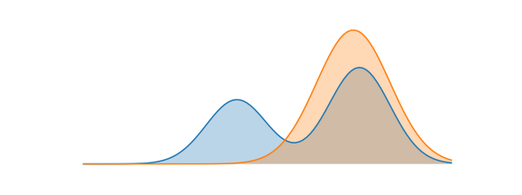
• Reverse KL is mode-seeking: the policy concentrates on high-probability regions of $p$, possibly sacrificing diversity.
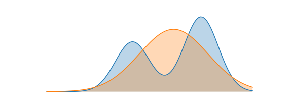
• Forward KL is mass-covering: the policy tries to cover the support of $p$.

RLHF typically uses reverse KL because we want the actor not to stray too far from the reference, rather than requiring it to cover every mode.

1.2 First Fix the Problem With Three Questions

The choices behind a KL-penalty implementation boil down to three questions: who the samples come from, which KL direction you want to constrain, and whether the KL term is backpropagated directly or only used as a reward coefficient. Change any one answer, and the recommended estimator may change too:

Scope: This post focuses on token/sample-level KL terms and their behavior inside the main policy-gradient term. I only comment briefly on learned critics, GAE, baseline normalization, and fully rigorous off-policy correction for general multi-step MDPs.

Unlike classic notes that mainly discuss KL approximation as a value-estimation problem, this post is closer to the recent LLM-RL question of gradient correctness: once the same estimator moves from a reward coefficient to a differentiable loss term, is it still optimizing the objective you think it is? These three questions determine all recommendations below; the main mental model is:

$$ \text{KL value estimator} \neq \text{KL optimization objective} \neq \text{gradient actually returned by code}. $$

The rest of the post repeatedly checks whether these three objects coincide — in most “wrong” configurations the issue is not a slightly worse value estimate, but a gradient target that has quietly changed. The operational answers are condensed into the three cheat-sheet tables in the next section.

2. Cheat Sheet (Skim-and-Go)

The three tables below condense the entire operational guidance of the post. A minimal notation primer is given first so you can read them, pick the recommended writing for your setting, and dive back into the derivations later.

Notation primer (full definitions in the next chapter):

• $q_\theta$: current policy; $p$: reference policy; $\mu$: sampling policy (on-policy means $\mu = q_\theta$).
• $k_1 = \log\frac{q_\theta}{p}$, $k_2 = \frac{1}{2}\left(\log\frac{p}{q_\theta}\right)^2$, $k_3 = \frac{p}{q_\theta} - 1 - \log\frac{p}{q_\theta}$.
• $\rho = \frac{q_\theta}{\text{sg}(\mu)}$: unified importance weight; $\text{sg}(\cdot)$ is stop-gradient.

2.1 On-Policy Reverse KL as a Loss Term

Note: $k_2$ and $\frac{q_\theta}{\text{sg}(q_\theta)} k_3$ have identical gradients (sample-level equivalent). For on-policy, directly using $k_2$ is recommended as the simplest approach.

2.2 Off-Policy Reverse KL as a Loss Term

Note: $\text{sg}\left(\frac{q_\theta}{\mu}\right) k_2$ and $\frac{q_\theta}{\mu} k_3$ have identical gradients (sample-level equivalent). Both are recommended choices.

2.3 KL as Reward Shaping (stop-gradient)

Note: For the stop-gradient reward-shaping setup analyzed here, only $k_1$ keeps the policy-gradient term aligned with reverse-KL regularization. Both $k_2$ and $k_3$ introduce bias in that term; even though $k_3$ is value-unbiased with low variance, it theoretically already deviates from the target gradient.

Legend: ✓✓ strongly recommended; ✓ recommended (slightly more complex or minor drawback); △ usable with caution; ✗✗ does not match the objective discussed here.

For derivations, variance analysis, and common pitfalls, keep reading.

3. Preliminaries: Notation and Basic Concepts

Before getting into the analysis, let’s fix the notation and write down two basic results that will be used throughout.

3.1 Notation, Sampling Distribution, and the True Gradient of the Objective

Notation:

• $q_\theta$: Current actor policy (parameterized by $\theta$)
• $q$: When unambiguous, we write $q := q_\theta$
• $p$: Reference policy (independent of $\theta$)
• $\mu$: Behavior policy for off-policy sampling (independent of $\theta$)
• $s_\theta(x) = \nabla_\theta \log q_\theta(x)$: Score function
• $\text{sg}(\cdot)$: Stop-gradient operation (.detach() in code)

A Unified Perspective on Sampling Policies: Introducing the $\rho$ Notation

When analyzing KL-estimator gradients, on-policy and off-policy may look like separate cases, but they can be handled in one framework.

Introduce the sampling policy $\mu$, meaning data are drawn from $x \sim \mu$. Define the unified ratio:

$$ \rho(x) := \frac{q_\theta(x)}{\text{sg}(\mu(x))} $$

The key insight is: in both on-policy and off-policy analyses, we treat the sampling policy $\mu$ as a gradient constant (i.e., apply stop-gradient to $\mu$).

• Off-policy ($\mu \neq q_\theta$): $\mu$ is inherently independent of $\theta$, so $\text{sg}(\mu) = \mu$, giving $\rho = \frac{q_\theta}{\mu}$
• On-policy ($\mu = q_\theta$): Set $\mu = q_\theta$ but stop its gradient, so $\rho = \frac{q_\theta}{\text{sg}(q_\theta)} \equiv 1$ (numerically always 1), while still having $\nabla_\theta \rho = s_\theta \neq 0$

In the on-policy case, even though $\rho \equiv 1$ numerically, you must explicitly construct $\rho = \frac{q_\theta}{\text{sg}(q_\theta)}$ (or equivalently $\rho = \exp(\log q_\theta - \text{sg}(\log q_\theta))$) in the computation graph: what it restores is the gradient path coming from the sampling distribution’s dependence on $\theta$ — the exact reason why expect-then-differentiate and differentiate-then-expect can disagree on-policy. Replace it with the literal constant 1, and that path is gone; the derivation degenerates to the “naive on-policy implementation” described later.

With this notation in place, the rest of the derivation no longer needs two separate tracks.

Score Function and True KL Gradients

The score function has an important property: $\mathbb{E}_{q_\theta}[s_\theta] = 0$ (since $\int \nabla_\theta q_\theta dx = \nabla_\theta \int q_\theta dx = \nabla_\theta 1 = 0$).

Using this property, we can derive the true gradients of forward and reverse KL divergences with respect to $\theta$.

Reverse KL Gradient:

$$ D_{\mathrm{KL}}(q_\theta \| p) = \int q_\theta(x) \log \frac{q_\theta(x)}{p(x)} dx $$

Differentiating with respect to $\theta$ (using the product rule):

$$ \nabla_\theta D_{\mathrm{KL}}(q_\theta \| p) = \int \nabla_\theta q_\theta \cdot \log \frac{q_\theta}{p} dx + \int q_\theta \cdot \nabla_\theta \log \frac{q_\theta}{p} dx $$

Using $\nabla_\theta q_\theta = q_\theta \cdot s_\theta$, $\nabla_\theta \log q_\theta = s_\theta$, and $\nabla_\theta \log p = 0$:

$$ = \mathbb{E}_{q_\theta}\left[s_\theta \cdot \log \frac{q_\theta}{p}\right] + \int q_\theta(x) \cdot s_\theta(x)\, dx \\ = \mathbb{E}_{q_\theta}\left[s_\theta \cdot \log \frac{q_\theta}{p}\right] + \mathbb{E}_{q_\theta}[s_\theta] \\ = \mathbb{E}_{q_\theta}\left[s_\theta \cdot \log \frac{q_\theta}{p}\right] $$

Thus:

$$ \boxed{\nabla_\theta D_{\mathrm{KL}}(q_\theta \| p) = \mathbb{E}_{q_\theta}\left[s_\theta \cdot \log \frac{q_\theta}{p}\right] = -\mathbb{E}_{q_\theta}\left[s_\theta \cdot \log \frac{p}{q_\theta}\right]} $$

Preview: We will later define $k_1 := -\log\frac{p}{q_\theta}$, so the above can be written concisely as $\nabla_\theta D_{\mathrm{KL}}(q_\theta \| p) = \mathbb{E}_{q_\theta}[s_\theta \cdot k_1]$ — this form appears repeatedly in gradient analysis.

Forward KL Gradient:

$$ D_{\mathrm{KL}}(p \| q_\theta) = \int p(x) \log \frac{p(x)}{q_\theta(x)} dx $$

Since $p(x)$ is independent of $\theta$:

$$ \nabla_\theta D_{\mathrm{KL}}(p \| q_\theta) = \int p(x) \cdot \nabla_\theta \left(-\log q_\theta(x)\right) dx = -\mathbb{E}_p[s_\theta] $$

To estimate this using samples from $q$, apply importance sampling:

$$ -\mathbb{E}_p[s_\theta] = -\mathbb{E}_{q_\theta}\left[\frac{p}{q_\theta} \cdot s_\theta\right] = \mathbb{E}_{q_\theta}\left[\left(1-\frac{p}{q_\theta}\right) \cdot s_\theta\right] $$

where the last step uses $\mathbb{E}_{q_\theta}[s_\theta] = 0$. Therefore

$$ \boxed{\nabla_\theta D_{\mathrm{KL}}(p \| q_\theta) = \mathbb{E}_{q_\theta}\left[\left(1-\frac{p}{q_\theta}\right) \cdot s_\theta\right]} $$

Preview: We will later derive $\nabla_\theta k_3 = (1-\frac{p}{q_\theta}) s_\theta$, so $\mathbb{E}_{q_\theta}[\nabla_\theta k_3] = \nabla_\theta D_{\mathrm{KL}}(p \| q_\theta)$ (forward KL). This is why directly backpropagating through $k_3$ produces the “wrong” gradient direction when you intend reverse KL.

With these two results, we can later determine which KL’s true gradient each estimator’s gradient expectation corresponds to.

4. Three Estimators: Definitions and Design Principles

Let $\frac{p(x)}{q_\theta(x)}$ denote the ratio. In a classic note, John Schulman compared three single-sample KL estimators that keep showing up in RLHF and LLM-RL implementations.

4.1 The Three Estimators: Definitions and Intuition

$k_1$: The Naive Log-Ratio Estimator

$$ k_1(x) = -\log \frac{p(x)}{q_\theta(x)} = \log q_\theta(x) - \log p(x) $$

This is the most direct definition: the negative log-ratio. It is unbiased for reverse KL, but the main issue is not that it targets the wrong thing. The issue is that a single sample can be positive or negative. Even when the true KL is small, samples can still swing in both directions, which often leads to large relative variance.

$k_2$: The Squared Log-Ratio Estimator

$$ k_2(x) = \frac{1}{2}\left(\log \frac{p(x)}{q_\theta(x)}\right)^2 $$

Design motivation: $k_1$ can be either positive or negative; squaring yields an estimator where every sample is non-negative, and each sample measures the magnitude of mismatch between $p$ and $q$.

Why is the bias often small? More precisely, $\mathbb{E}_{q_\theta}[k_2]$ is not reverse KL itself, but near $q_\theta \approx p$ it shares the same second-order local expansion. So it is best understood as a locally useful surrogate; once you leave that small-KL neighborhood, the approximation need not stay reliable.

Technical note: why does $k_2$ share the same second-order local behavior as reverse KL?

Under the usual regularity conditions, if $q_{\theta_0}=p$ and we perturb by a small $\Delta\theta$, then

$$ \mathbb{E}_{q_{\theta_0+\Delta\theta}}[k_2] = \frac{1}{2}\, \Delta\theta^T F(\theta_0)\, \Delta\theta + O(\|\Delta\theta\|^3), $$

and

$$ D_{\mathrm{KL}}\big(q_{\theta_0+\Delta\theta} \| p\big) = \frac{1}{2}\, \Delta\theta^T F(\theta_0)\, \Delta\theta + O(\|\Delta\theta\|^3), $$

where $F(\theta_0)$ is the Fisher information matrix at $\theta_0$.

$k_3$: The Bregman Divergence Estimator via Control Variates

$$ k_3(x) = \frac{p(x)}{q_\theta(x)} - 1 - \log \frac{p(x)}{q_\theta(x)} $$

Design motivation: We want an estimator that is both unbiased and low variance. A standard approach is to add a control variate to $k_1$—a term with zero expectation that (ideally) is negatively correlated with $k_1$.

Note that $\mathbb{E}_{q_\theta}\left[\frac{p}{q_\theta} - 1\right] = \mathbb{E}_{q_\theta}\left[\frac{p}{q_\theta}\right] - 1 = 1 - 1 = 0$, so for any $\lambda$,

$$ k_1 + \lambda\left(\frac{p}{q_\theta} - 1\right) = -\log \frac{p}{q_\theta} + \lambda\left(\frac{p}{q_\theta} - 1\right) $$

remains an unbiased estimator.

Why choose $\lambda = 1$? Since $\log$ is concave, we have $\log x \leq x - 1$, therefore

$$ k_3 = \left(\frac{p}{q_\theta} - 1\right) - \log \frac{p}{q_\theta} \geq 0 $$

It is always non-negative. This ensures every sample contributes “positively” to the estimate, eliminating the cancellation problem of $k_1$.

Geometric intuition: $k_3$ is actually a Bregman divergence. Consider the convex function $\phi(x) = -\log x$, whose tangent at $x=1$ is $y = 1 - x$. The Bregman divergence is defined as the difference between the function value and the tangent value:

$$ \begin{aligned} D_\phi\left(\frac{p}{q_\theta}, 1\right) &= \phi\left(\frac{p}{q_\theta}\right) - \phi(1) - \phi'(1)\left(\frac{p}{q_\theta} - 1\right) \\ &= -\log \frac{p}{q_\theta} - 0 - (-1)\left(\frac{p}{q_\theta} - 1\right) \\ &= \frac{p}{q_\theta} - 1 - \log \frac{p}{q_\theta} \\ &= k_3. \end{aligned} $$

Since a convex function always lies above its tangent, this gap is naturally non-negative. More importantly, as $\frac{p}{q_\theta} \to 1$, the gap shrinks at a second-order rate $\left(\frac{p}{q_\theta} - 1\right)^2$, which is the fundamental reason why $k_3$ tends to have lower variance when the policies are close.

A third reading (unnormalized KL): RPG (Zhang et al., 2025) points out that $k_3$ is exactly the integrand of the unnormalized (generalized) KL $D(\tilde q \| \tilde p) = \int \tilde q \log \frac{\tilde q}{\tilde p} - \int \tilde q + \int \tilde p$: expanding pointwise for normalized $q, p$ gives $q \cdot \left[\log\frac{q}{p} + \frac{p}{q} - 1\right] = q \cdot k_3$. The standard KL integrand $q\log\frac{q}{p}$ can be negative pointwise, while this one is pointwise non-negative — the control-variate, Bregman, and unnormalized-KL readings are three views of the same construction.

The design logic is easiest to see side by side:

Before discussing bias, variance, and gradients, separate the usage semantics: the same $k_i$ can serve as a value metric (all that matters is its expectation and variance), as a differentiable loss (what matters is which objective its backpropagated gradient follows), or as a reward-shaping coefficient (what matters is the policy gradient it induces). When the post says a configuration is “correct” or “incorrect,” it is about the gradient induced under that usage, not about whether the scalar sample can estimate a KL value.

5. Value Estimation: Bias and Variance

Assume we sample from $q_\theta$ to estimate reverse KL $D_{\mathrm{KL}}(q_\theta \| p)$:

5.1 Unbiasedness Analysis

$$ \begin{aligned} \mathbb{E}_{q_\theta}[k_1] &= \mathbb{E}_{q_\theta}\left[\log \tfrac{q_\theta}{p}\right] = D_{\mathrm{KL}}(q_\theta \| p) && \textbf{(unbiased)} \\[8pt] \mathbb{E}_{q_\theta}[k_3] &= \mathbb{E}_{q_\theta}\left[\frac{p}{q_\theta} - 1 - \log \frac{p}{q_\theta}\right] && \\ &= 1 - 1 + D_{\mathrm{KL}}(q_\theta \| p) && \\ &= D_{\mathrm{KL}}(q_\theta \| p) && \textbf{(unbiased)} \\[8pt] \mathbb{E}_{q_\theta}[k_2] &= \frac{1}{2}\mathbb{E}_{q_\theta}\left[\left(\log \frac{p}{q_\theta}\right)^2\right] \neq D_{\mathrm{KL}}(q_\theta \| p) && \textbf{(biased)} \end{aligned} $$

For reverse KL values, $k_1$ and $k_3$ are unbiased estimators, while $k_2$ is biased.

5.2 Variance Characteristics

John Schulman’s numerical examples ($q = \mathcal{N}(0,1)$, $p = \mathcal{N}(0.1,1)$, true KL = 0.005) show:

When KL is large ($p = \mathcal{N}(1,1)$, true KL = 0.5):

Intuitively:

• $k_1 = -\log \frac{p}{q}$ has a first-order term; when $\frac{p}{q}$ is close to 1 it can fluctuate substantially and can be negative.
• $k_3 = \frac{p}{q} - 1 - \log \frac{p}{q}$ is second-order around $\frac{p}{q}=1$ and is always non-negative, which typically yields lower variance when the policies are close.
• Once you leave the small-KL, well-covered regime and $\frac{p}{q}$ can become very large, the variance of $k_3$ can also blow up: locally $k_3 \approx \frac{1}{2}\left(\frac{p}{q} - 1\right)^2$, whose expectation is half the $\chi^2$ divergence $\chi^2(p \| q)$ — exactly the quantity that diverges under poor coverage. At that point the comparison between $k_1$ and $k_3$ is no longer one-sided.

At the pure value-estimation level: $k_1$ is unbiased but high-variance, $k_2$ is low-variance but biased, and $k_3$ is unbiased, always positive, and low-variance. So in the common small-KL, well-covered regime, $k_3$ is often the safest choice when only values matter.

Note: To estimate the forward KL value $D_{\mathrm{KL}}(p \| q_\theta) = \mathbb{E}_p\left[\log \frac{p}{q_\theta}\right]$ while only sampling from $q_\theta$, importance sampling gives $\mathbb{E}_{q_\theta}[r \log r]$ with $r = \frac{p}{q_\theta}$. Schulman’s note goes one step further and subtracts the zero-mean control variate $r - 1$, giving $\mathbb{E}_{q_\theta}[r \log r - (r - 1)]$: still unbiased, but always non-negative and lower variance (the same Bregman construction as $k_3$, applied to $f(x) = x \log x$).

6. Two Ways to Use a KL Penalty

The next fork in the road is simply how the KL penalty is used in code. That choice determines whether value-estimation properties are enough, or whether gradient properties become the real issue.

Recall the objective for KL-regularized reinforcement learning ($\tau \sim q_\theta$ denotes the trajectory distribution induced by policy $q_\theta$, and $\beta > 0$ is the penalty coefficient):

$$ J(\theta) = \mathbb{E}_{\tau \sim q_\theta} \left[ \sum_{t=0}^T \gamma^t r(s_t, a_t) \right] - \beta \cdot D_{\mathrm{KL}}(q_\theta \| p) $$

A quick bridge to the token-level analysis below: when the two policies share the same environment transitions (in LLM RL, the same context-building process), the trajectory-level KL decomposes exactly (for $\gamma = 1$) into the expected sum of per-token conditional KLs. The token-level KL terms that implementations penalize are that decomposition in code form.

This mathematical form looks unified, but in actor-critic algorithms (e.g., PPO) it gives rise to two fundamentally different implementation paradigms. They often differ by only a few lines of code, yet correspond to different optimization semantics.

Notation: In this section, we use $\text{KL}_t$ or $\text{KL}(s)$ to generically refer to a token/state-level KL estimator (such as $k_1, k_2, k_3$), with specific definitions from the earlier section “Three Estimators: Definitions and Design Principles”.

6.1 As a Loss Term: KL Backpropagates Directly

actor_loss = -advantage * log_prob + beta * kl  # kl participates in gradient

The critic learns only the environment value function; the KL term acts as an explicit regularizer for the actor and participates directly in backpropagation.

6.2 As a Reward-Shaping Term: KL Changes Reward but Does Not Backpropagate

kl = compute_kl(log_prob_q, log_prob_p).detach()
shaped_reward = reward - beta * kl

KL is treated as part of the reward via reward shaping, and the actor-critic update is performed on the shaped reward. The KL term itself is detached and does not backpropagate.

In many implementations, these two forms differ by just a .detach(). But optimization-wise they are not the same algorithm. The basic split is:

• KL as a loss term: Requires correct gradients for the KL component, including which objective those gradients correspond to.
• KL as a reward-shaping term: Requires accurate KL values, and also requires that the induced policy-gradient update matches the intended objective.

7. Gradient Analysis for Differentiable KL Losses

When KL serves as a differentiable loss term, the key question is which objective each estimator actually optimizes through its gradient. This is subtle but central to the theory.

We keep using the unified weight $\rho = \frac{q_\theta}{\text{sg}(\mu)}$ from Section 3.1, so on-policy and off-policy can be handled in one derivation. In both cases $\nabla_\theta \rho = \rho \cdot s_\theta$: off-policy, $\rho = \frac{q_\theta}{\mu}$; on-policy, $\rho \equiv 1$ numerically, yet the gradient $\nabla_\theta \rho = s_\theta$ is nonzero.

7.1 Basic Gradients of the Three Estimators

First, we compute the gradients of the three estimators themselves (without $\rho$). These results will be used repeatedly in subsequent analysis.

Deriving $\nabla_\theta k_1$: from $k_1 = \log q_\theta(x) - \log p(x)$ and $\nabla_\theta \log p = 0$,

$$ \nabla_\theta k_1 = \nabla_\theta \log q_\theta(x) = s_\theta $$

Deriving $\nabla_\theta k_2$:

$$ k_2 = \frac{1}{2}\left(\log \frac{p}{q_\theta}\right)^2 $$

By the chain rule:

$$ \begin{aligned} \nabla_\theta k_2 &= \left(\log \frac{p}{q_\theta}\right) \cdot \nabla_\theta\left(\log \frac{p}{q_\theta}\right) \\ &= \left(\log \frac{p}{q_\theta}\right) \cdot \nabla_\theta(\log p(x) - \log q_\theta(x)) \\ &= \left(\log \frac{p}{q_\theta}\right)(-s_\theta) \\ &= - \left(\log \frac{p}{q_\theta}\right) s_\theta. \end{aligned} $$

Deriving $\nabla_\theta k_3$:

$$ k_3 = \frac{p}{q_\theta} - 1 - \log \frac{p}{q_\theta} $$

First, compute $\nabla_\theta \frac{p}{q_\theta}$. Since $\frac{p}{q_\theta} = p(x) \cdot q_\theta(x)^{-1}$:

$$ \nabla_\theta \frac{p}{q_\theta} = p(x) \cdot (-1) \cdot q_\theta(x)^{-2} \cdot \nabla_\theta q_\theta(x) = -\frac{p(x)}{q_\theta(x)} \cdot \frac{\nabla_\theta q_\theta(x)}{q_\theta(x)} = -\frac{p}{q_\theta} \cdot s_\theta $$

Then compute $\nabla_\theta \log \frac{p}{q_\theta}$:

$$ \nabla_\theta \log \frac{p}{q_\theta} = \frac{q_\theta}{p} \nabla_\theta \frac{p}{q_\theta} = \frac{q_\theta}{p} \cdot \left(-\frac{p}{q_\theta} \cdot s_\theta\right) = -s_\theta $$

Therefore:

$$ \nabla_\theta k_3 = \nabla_\theta \frac{p}{q_\theta} - 0 - \nabla_\theta \log \frac{p}{q_\theta} = -\frac{p}{q_\theta} \cdot s_\theta - (-s_\theta) = \left(1 - \frac{p}{q_\theta}\right) \cdot s_\theta $$

The gradients of the three estimators are:

• $\nabla_\theta k_1 = s_\theta$
• $\nabla_\theta k_2 = -\left(\log \frac{p}{q_\theta}\right) s_\theta = k_1 \cdot s_\theta$
• $\nabla_\theta k_3 = \left(1 - \frac{p}{q_\theta}\right) s_\theta$

These basic gradients will be used repeatedly in the unified framework analysis that follows.

“The Gradient of the Mathematical Objective” vs. “The Gradient Returned by Code”

When analyzing estimator gradients, there is a common pitfall: “expect-then-differentiate” and “differentiate-then-expect” need not agree.

If we treat $\mathbb{E}_{q_\theta}[k_i]$ as a function of $\theta$ and differentiate analytically (i.e., “expect-then-differentiate”), then because $\mathbb{E}_{q_\theta}[k_1] = \mathbb{E}_{q_\theta}[k_3] = D_{\mathrm{KL}}(q_\theta \| p)$, we have:

$$ \nabla_\theta \mathbb{E}_{q_\theta}[k_1] = \nabla_\theta D_{\mathrm{KL}}(q_\theta \| p) $$

$$ \nabla_\theta \mathbb{E}_{q_\theta}[k_3] = \nabla_\theta D_{\mathrm{KL}}(q_\theta \| p) $$

Both yield the reverse-KL gradient. However, when you backpropagate through the sample mean of $k_i$ in code, autograd effectively computes “differentiate-then-expect”, i.e., $\mathbb{E}_{q_\theta}[\nabla_\theta k_i]$, which can differ.

The root cause is that the sampling distribution $q_\theta$ depends on $\theta$, so expectation and differentiation cannot be exchanged naively. This is exactly the subtlety in the on-policy case, and why we introduce the unified $\rho$ framework.

7.2 Gradient Analysis Under the Unified Framework

Now, we use the $\rho$ framework to uniformly handle on-policy and off-policy scenarios. Consider the loss function form $L = \rho \cdot k$, where $\rho = \frac{q_\theta}{\text{sg}(\mu)}$. (Throughout, assume $\mu$ covers $q_\theta$, i.e. $\mathrm{supp}(q_\theta) \subseteq \mathrm{supp}(\mu)$, so that $\rho$ is well-defined.)

From here on, every expectation is with respect to a fixed sampling distribution $\mu$. Because $\mu$ does not depend on $\theta$, differentiation and expectation can be exchanged freely (the warning of the previous section only concerns $\mathbb{E}_{q_\theta}[\cdot]$):

$$ \nabla_\theta \mathbb{E}_{\mu}[f_\theta(x)] = \mathbb{E}_{\mu}[\nabla_\theta f_\theta(x)] $$

Gradient Derivations for the Three Estimators Under the Unified Framework

Using $\nabla_\theta \rho = \rho \cdot s_\theta$ (since $\rho = q_\theta / \text{sg}(\mu)$), combined with the previously derived $\nabla_\theta k_i$, applying the product rule:

$\nabla_\theta(\rho k_1)$:

$$ \nabla_\theta(\rho k_1) = (\nabla_\theta \rho) k_1 + \rho (\nabla_\theta k_1) = \rho s_\theta k_1 + \rho s_\theta = \rho s_\theta (k_1 + 1) $$

$\nabla_\theta(\rho k_2)$:

$$ \nabla_\theta(\rho k_2) = \rho s_\theta k_2 + \rho \left(-\log \frac{p}{q_\theta}\right) s_\theta = \rho s_\theta \left(k_2 - \log \frac{p}{q_\theta}\right) = \rho s_\theta (k_2 + k_1) $$

$\nabla_\theta(\text{sg}(\rho) k_2)$ (applying stop-gradient to $\rho$):

$$ \nabla_\theta(\text{sg}(\rho) k_2) = \text{sg}(\rho) \cdot \nabla_\theta k_2 = \rho \cdot \left(-\log \frac{p}{q_\theta}\right) s_\theta = \rho s_\theta k_1 $$

$\nabla_\theta(\rho k_3)$:

$$ \nabla_\theta(\rho k_3) = \rho s_\theta k_3 + \rho \left(1-\frac{p}{q_\theta}\right) s_\theta = \rho s_\theta \left(k_3 + 1 - \frac{p}{q_\theta}\right) $$

Substituting $k_3 = \frac{p}{q_\theta} - 1 - \log \frac{p}{q_\theta}$:

$$ k_3 + 1 - \frac{p}{q_\theta} = \left(\frac{p}{q_\theta} - 1 - \log \frac{p}{q_\theta}\right) + 1 - \frac{p}{q_\theta} = -\log \frac{p}{q_\theta} = k_1 $$

Here the algebra collapses in an important way:

$$ \boxed{\nabla_\theta(\rho k_3) = \rho s_\theta k_1} $$

Gradient Expectations and Optimization Objectives

Using $\mathbb{E}_\mu[\rho \cdot f] = \mathbb{E}_{q_\theta}[f]$ and $\mathbb{E}_{q_\theta}[s_\theta] = 0$:

$\mathbb{E}_\mu[\nabla_\theta(\rho k_1)]$:

$$ \mathbb{E}_\mu[\rho s_\theta (k_1 + 1)] = \mathbb{E}_{q_\theta}[s_\theta k_1] + \underbrace{\mathbb{E}_{q_\theta}[s_\theta]}_{=0} = \nabla_\theta D_{\mathrm{KL}}(q_\theta \| p) \quad \checkmark $$

$\mathbb{E}_\mu[\nabla_\theta(\rho k_2)]$:

$$ \begin{aligned} \mathbb{E}_\mu[\rho s_\theta (k_2 + k_1)] &= \mathbb{E}_{q_\theta}[s_\theta k_2] + \mathbb{E}_{q_\theta}[s_\theta k_1] \\ &= \mathbb{E}_{q_\theta}[s_\theta k_2] + \mathbb{E}_{q_\theta}[\nabla_\theta k_2] && \text{(since } \nabla_\theta k_2 = k_1 s_\theta \text{)} \\ &= \nabla_\theta \mathbb{E}_{q_\theta}[k_2] && \text{(recombining score-function and direct-gradient terms)} \end{aligned} $$

In other words, the gradient expectation of $\rho k_2$ corresponds to “minimizing $\mathbb{E}_{q_\theta}[k_2]$” (a surrogate with the same local second-order behavior as KL), not the true gradient of reverse KL $D_{\mathrm{KL}}(q_\theta\|p)$; therefore, when the goal is to optimize reverse KL exactly, avoid using $\rho k_2$. (The gap to the true reverse-KL gradient is $\mathbb{E}_{q_\theta}[s_\theta k_2]$ — a higher-order small term near $q_\theta \approx p$, but uncontrolled once you leave that neighborhood.)

$\mathbb{E}_\mu[\nabla_\theta(\text{sg}(\rho) k_2)]$ and $\mathbb{E}_\mu[\nabla_\theta(\rho k_3)]$ (their gradient random variables are the same, $\rho s_\theta k_1$):

$$ \mathbb{E}_\mu[\rho s_\theta k_1] = \mathbb{E}_{q_\theta}[s_\theta k_1] = \nabla_\theta D_{\mathrm{KL}}(q_\theta \| p) \quad \checkmark $$

Gradient Equivalence: Which Methods Produce Identical Gradient Random Variables

This is also why $\text{sg}(\rho) k_2$ and $\rho k_3$ keep appearing together: for the same sample $x$, they backpropagate the exact same gradient vector, namely $\rho s_\theta k_1$. Not just the same expectation - the same sample-level gradient. So their means, variances, and higher-order statistics all match.

7.3 A Unified View of On-Policy and Off-Policy

With that in place, the on-policy/off-policy relationship becomes much easier to read.

On-policy ($\mu = q_\theta$):

• $\rho = \frac{q_\theta}{\text{sg}(q_\theta)} \equiv 1$ (numerically always 1)
• $\rho k_1 = k_1$, $\rho k_2 = k_2$, $\rho k_3 = k_3$
• But the gradients differ, because $\nabla_\theta \rho = s_\theta \neq 0$.

This explains why naive direct backpropagation (i.e., without explicitly constructing $\rho$) fails when using $k_1$ or $k_3$ as the KL loss term in the on-policy case:

• Directly using $k_1$ (without $\rho$): $\mathbb{E}_{q_\theta}[\nabla k_1] = \mathbb{E}_{q_\theta}[s_\theta] = 0$, so the KL term is ineffective.
• Directly using $k_3$ (without $\rho$): $\mathbb{E}_{q_\theta}[\nabla k_3] = \nabla D_{\mathrm{KL}}(p \| q_\theta)$ (forward KL), i.e., the wrong direction for reverse-KL regularization.
• Directly using $k_2$: $\mathbb{E}_{q_\theta}[\nabla k_2] = \nabla D_{\mathrm{KL}}(q_\theta \| p)$ (reverse KL), which makes it the only choice consistent with the target under the naive implementation.

A real-world instance: the original GRPO objective (DeepSeekMath, Eq. 3–4) adds exactly this naive on-policy $k_3$ as a differentiable loss term — in verl this corresponds to kl_loss_type=low_var_kl. By the decomposition above, the expected gradient of that KL term points along forward KL $D_{\mathrm{KL}}(p \| q_\theta)$, not the reverse KL written in the objective; recent analyses such as Rethinking KL Regularization in RLHF (Liu et al., 2025) and A Comedy of Estimators (Shah et al., 2025) make the same observation. Two fixes exist: DeepSeek-V3.2 adopts the importance-ratio-corrected $\rho k_3$ (Section 7.4), and verl’s k3+ option (report the $k_3$ value, backpropagate through $k_2$ via straight-through) implements the same idea differently.

If you explicitly construct $\rho = \frac{q_\theta}{\text{sg}(q_\theta)}$ (on-policy), or use the standard importance weight $\rho = \frac{q_\theta}{\mu}$ (off-policy, $\mu \neq q_\theta$), the same conclusions hold in both cases:

• Usable: $\rho k_1$ (higher variance), $\text{sg}(\rho) k_2$ (recommended), and $\rho k_3$ (recommended) all yield reverse-KL gradients.
• Not suitable for exactly optimizing reverse KL: $\rho k_2$ (where $\rho$ participates in the gradient) — it optimizes a local second-order surrogate instead.

The reason $k_2$ works directly in the on-policy case is not a general principle; it is a special degeneration when $\rho \equiv 1$. In that setting, $\nabla_\theta k_2 = k_1 s_\theta$ happens to land on the correct reverse-KL gradient. That should not be extrapolated to general off-policy settings.

For an in-depth analysis of off-policy scenarios in large language models, refer to my previous blog post: From Two-Policy to Three-Policy: TRPO Extension Under Behavior-Reference Mismatch in LLM RL.

7.4 Variance Analysis

Earlier we saw that three choices give unbiased gradients for reverse KL: $\rho k_1$, $\text{sg}(\rho) k_2$, $\rho k_3$. Their gradient random variables are (note that $s_\theta$ is a vector, so the gradient is also a vector):

$$ g_1(x) = \rho(x) s_\theta(x) (k_1(x) + 1), \quad g_\star(x) = \rho(x) s_\theta(x) k_1(x) $$

where $g_\star$ corresponds to both $\text{sg}(\rho) k_2$ and $\rho k_3$ (they are identical).

To avoid ambiguity in “variance of a vector gradient”, we compare the projection variance in any direction: take any unit vector $u$, and define scalar random variables

$$ g_1^{(u)} := u^\top g_1, \quad g_\star^{(u)} := u^\top g_\star. $$

Let $A_u(x) := \rho(x)\, u^\top s_\theta(x)$, $B(x) := k_1(x)$, then

$$ g_1^{(u)} = A_u(B+1), \quad g_\star^{(u)} = A_u B. $$

Both have the same expectation, and the variance difference in any direction is

$$ \boxed{ \mathrm{Var}_\mu\big(g_1^{(u)}\big) - \mathrm{Var}_\mu\big(g_\star^{(u)}\big) = \mathbb{E}_\mu\big[A_u(x)^2 \big(2B(x)+1\big)\big] = \mathbb{E}_\mu\Big[\rho(x)^2\,\big(u^\top s_\theta(x)\big)^2\,\big(2k_1(x)+1\big)\Big]. } $$

In the typical KL penalty regime ($q_\theta \approx p \approx \mu$), setting $\frac{p(x)}{q_\theta(x)} = 1 + \varepsilon(x)$, $|\varepsilon| \ll 1$:

• $k_1 = -\log \frac{p}{q_\theta} \approx -\varepsilon$
• $2k_1 + 1 \approx 1 - 2\varepsilon$, with the leading term being a positive $O(1)$ constant

Therefore $\mathrm{Var}_\mu(g_1) > \mathrm{Var}_\mu(g_\star)$.

Once you leave this small-KL neighborhood, however, the sign of $2k_1+1$ is no longer guaranteed. At that point the comparison also depends on the $\rho^2$ weighting and the score-function term, so the local expansion above should not be over-interpreted.

Intuitively: $g_1 = \rho s_\theta (k_1 + 1)$ carries an extra zero-mean noise term $\rho s_\theta$ of magnitude $O(1)$, while $g_\star = \rho s_\theta k_1$ keeps only a first-order term proportional to $\varepsilon$ — which is why $\rho k_1$ is usually noisier in the typical small-KL regime.

Practical recommendation: For optimizing reverse KL, prefer $\rho k_3$ or $\text{sg}(\rho) k_2$ (both have equivalent gradients and low variance); $\rho k_1$ is unbiased but has higher variance, and can serve as a fallback with clipping/regularization.

Warning (extreme off-policy mismatch):

When $\mu$ differs greatly from $q_\theta$ — for example, when $\mu$ has almost no samples in high-density regions of $q_\theta$, or when $\rho = q_\theta / \mu$ explodes in the tails — any $\rho$-based method will suffer from severe variance issues. In such cases, the advantage of $\rho k_3$ (or $\text{sg}(\rho) k_2$) over $\rho k_1$ is no longer theoretically guaranteed, and strategies like clipping and regularization must be combined.

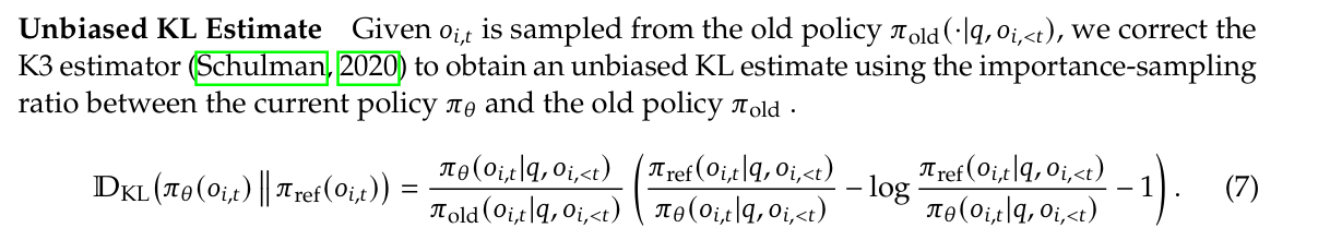
In the local-policy-update regime usually assumed here — KL controlled, sampling from a nearby policy $\mu = q_{\theta_\text{old}}$ — the recommendation above stands as stated. This is also how the DeepSeek-V3.2 technical report’s “unbiased KL estimate” lines up with the notation here: it uses $\frac{q_\theta}{\mu} k_3$, i.e. $\rho k_3$, recovering both unbiased KL estimation and the correct reverse-KL gradient — in the language of this post, precisely the fix for the naive $k_3$ loss inherited from GRPO-style objectives.

Gradient Summary

Under the unified framework, the gradient targets are:

where $\rho = \frac{q_\theta}{\text{sg}(\mu)}$. When on-policy ($\mu = q_\theta$), $\rho \equiv 1$.

It must be emphasized: the conclusions in the table above apply to the unified framework where the loss is written as $L=\rho\,k$ and $\rho$ retains its gradient path in the computation graph. On-policy, $\rho \equiv 1$ numerically, yet $\nabla_\theta \rho = s_\theta \neq 0$ — so $\rho k$ and “directly backpropagating through the sample mean of $k$” are not the same gradient. Drop the explicit $\rho$, and you fall back to the naive on-policy behavior at the start of Section 7.3: $k_1$ ineffective, $k_2$ reverse KL, $k_3$ forward KL.

8. Gradient Analysis for KL Reward Shaping

This is where the easiest mistake happens. Since both $k_1$ and $k_3$ are unbiased as reverse-KL value estimators, it is tempting to think that either one should be fine once detached and used inside reward shaping.

That inference is wrong. Value unbiasedness does not imply gradient correctness inside reward shaping. Once KL becomes part of shaped reward, the relevant object is $\mathbb{E}[s_\theta \hat{k}]$, not $\mathbb{E}[\hat{k}]$.

8.1 The True KL-Regularized Policy Gradient

Consider the KL-regularized reinforcement learning objective:

$$ J(\theta) = \mathbb{E}_{q_\theta}[R] - \beta \cdot D_{\mathrm{KL}}(q_\theta \| p) $$

Its true gradient is:

$$ \nabla_\theta J = \mathbb{E}_{q_\theta}[s_\theta \cdot R] - \beta \cdot \nabla_\theta D_{\mathrm{KL}}(q_\theta \| p) $$

Using the result from the “Preliminaries” section, the reverse KL gradient is:

$$ \nabla_\theta D_{\mathrm{KL}}(q_\theta \| p) = \mathbb{E}_{q_\theta}\left[s_\theta \cdot \left(-\log \frac{p}{q_\theta}\right)\right] = \mathbb{E}_{q_\theta}[s_\theta \cdot k_1] $$

Therefore, the true KL-regularized policy gradient is:

$$ \nabla_\theta J = \mathbb{E}_{q_\theta}\left[s_\theta \cdot \left(R - \beta \cdot k_1\right)\right] $$

Gradient Form When Using Estimator $\hat{k}$

For the next few paragraphs, focus only on the policy-gradient term itself. I am not folding in extra effects from learned critics, GAE, baseline fitting error, or normalization. In that simplified setting, when we use some estimator $\hat{k}$ (with stop-gradient) inside reward shaping, the shaped reward is $\tilde{R} = R - \beta \cdot \text{sg}(\hat{k})$, and the policy gradient becomes:

$$ \nabla_\theta \tilde{J} = \mathbb{E}_{q_\theta}\left[s_\theta \cdot (R - \beta \cdot \hat{k})\right] $$

Unbiasedness condition: $\nabla_\theta \tilde{J} = \nabla_\theta J$ if and only if

$$ \mathbb{E}_{q_\theta}[s_\theta \cdot \hat{k}] = \mathbb{E}_{q_\theta}[s_\theta \cdot k_1] $$

Using $k_1$ as Penalty: Gradient Unbiased

When $\hat{k} = k_1$, the condition is automatically satisfied:

$$ \mathbb{E}_{q_\theta}[s_\theta \cdot k_1] = \mathbb{E}_{q_\theta}[s_\theta \cdot k_1] \quad \checkmark $$

Therefore, when $k_1$ is used in reward shaping, the induced policy gradient is unbiased. This is exactly the classic per-token KL reward of RLHF pipelines in the InstructGPT lineage.

Using $k_3$ as Penalty: Gradient Biased

When $\hat{k} = k_3 = \frac{p}{q_\theta} - 1 - \log \frac{p}{q_\theta}$:

$$ \mathbb{E}_{q_\theta}[s_\theta \cdot k_3] = \mathbb{E}_{q_\theta}\left[s_\theta \cdot \left(\frac{p}{q_\theta} - 1\right)\right] + \mathbb{E}_{q_\theta}\left[s_\theta \cdot \left(-\log \frac{p}{q_\theta}\right)\right] $$

The second term is exactly $\mathbb{E}_{q_\theta}[s_\theta \cdot k_1]$. The problem lies in the first term:

$$ \mathbb{E}_{q_\theta}\left[s_\theta \cdot \left(\frac{p}{q_\theta} - 1\right)\right] = \mathbb{E}_{q_\theta}\left[s_\theta \cdot \frac{p}{q_\theta}\right] - \underbrace{\mathbb{E}_{q_\theta}[s_\theta]}_{=0} = \mathbb{E}_{q_\theta}\left[s_\theta \cdot \frac{p}{q_\theta}\right] $$

This can be rewritten as:

$$ \mathbb{E}_{q_\theta}\left[s_\theta \cdot \frac{p}{q_\theta}\right] = \int q_\theta(x) \cdot \nabla_\theta \log q_\theta(x) \cdot \frac{p(x)}{q_\theta(x)} dx = \int p(x) \cdot \nabla_\theta \log q_\theta(x) dx = \mathbb{E}_p[s_\theta] $$

Using the forward KL gradient formula $\nabla_\theta D_{\mathrm{KL}}(p \| q_\theta) = -\mathbb{E}_p[s_\theta]$, we have:

$$ \mathbb{E}_{q_\theta}\left[s_\theta \cdot \frac{p}{q_\theta}\right] = -\nabla_\theta D_{\mathrm{KL}}(p \| q_\theta) $$

Therefore:

$$ \mathbb{E}_{q_\theta}[s_\theta \cdot k_3] = \underbrace{-\nabla_\theta D_{\mathrm{KL}}(p \| q_\theta)}_{\text{bias term}} + \nabla_\theta D_{\mathrm{KL}}(q_\theta \| p) $$

When $k_3$ is used in reward shaping, the gradient is biased, with the bias term equal to the negative of the forward KL gradient.

It is worth reading this bias term as an objective in its own right. By the decomposition above, the KL penalty contributes to the ascent direction

$$ -\beta\,\mathbb{E}_{q_\theta}[s_\theta \cdot k_3] = -\beta\,\nabla_\theta\left[D_{\mathrm{KL}}(q_\theta \| p) - D_{\mathrm{KL}}(p \| q_\theta)\right], $$

so the “penalty” actually being minimized is the difference $D_{\mathrm{KL}}(q_\theta \| p) - D_{\mathrm{KL}}(p \| q_\theta)$ — which is not a divergence and is unbounded below. Two Gaussian examples make the danger concrete (take $q_\theta = \mathcal{N}(\theta, \sigma_q^2)$, $p = \mathcal{N}(m, \sigma_p^2)$; along the mean direction the two KL gradients are $(\theta-m)/\sigma_p^2$ and $(\theta-m)/\sigma_q^2$):

• Cancellation and sign flips: with equal variances ($\sigma_q = \sigma_p$) the two gradients coincide and cancel exactly, so the KL part of the update is exactly zero in expectation — the penalty silently does nothing, even though the measured KL value is correct and positive; when the reference is broader ($\sigma_p > \sigma_q$) it gets worse, as the difference gradient $(\theta-m)\left(\sigma_p^{-2} - \sigma_q^{-2}\right)$ has the opposite sign of the true reverse-KL gradient and pushes the policy mean away from the reference.
• Collapse incentive: with equal means and $\sigma_q \to 0$, the penalty $D_{\mathrm{KL}}(q_\theta \| p) - D_{\mathrm{KL}}(p \| q_\theta) = 2\log\frac{\sigma_p}{\sigma_q} + \frac{\sigma_q^2}{2\sigma_p^2} - \frac{\sigma_p^2}{2\sigma_q^2}$ is dominated by $-\frac{\sigma_p^2}{2\sigma_q^2}$ and tends to $-\infty$ — the update is actively rewarded for collapsing onto the mode of $p$.

This conclusion follows from the gradient decomposition itself and does not depend on any particular experiment.

Using $k_2$ as Penalty: Also Biased

When $\hat{k} = k_2 = \frac{1}{2}k_1^2$, the KL part of the induced policy-gradient term becomes

$$ \mathbb{E}_{q_\theta}[s_\theta \cdot k_2] = \frac{1}{2}\mathbb{E}_{q_\theta}[s_\theta \cdot k_1^2], $$

which is generally not equal to $\mathbb{E}_{q_\theta}[s_\theta \cdot k_1]$. So $k_2$ is also biased when used inside reward shaping.

Off-Policy Scenario Conclusions

The above analysis assumes on-policy sampling. Does the conclusion change in off-policy scenarios?

Let samples come from behavior policy $\mu$, using importance-weighted policy gradient:

$$ \nabla_\theta \tilde{J} = \mathbb{E}_\mu\left[\frac{q_\theta}{\mu} \cdot s_\theta \cdot (R - \beta \cdot k)\right] $$

Using $\mathbb{E}_\mu[\frac{q_\theta}{\mu} \cdot f] = \mathbb{E}_{q_\theta}[f]$, this equals:

$$ = \mathbb{E}_{q_\theta}[s_\theta \cdot R] - \beta \cdot \mathbb{E}_{q_\theta}[s_\theta \cdot k] $$

The unbiasedness condition remains $\mathbb{E}_{q_\theta}[s_\theta \cdot k] = \mathbb{E}_{q_\theta}[s_\theta \cdot k_1]$, exactly the same as on-policy.

One point is worth making explicit here: in the token/sample-level off-policy policy-gradient term discussed in this post, the importance weight $\frac{q_\theta}{\mu}$ multiplies the whole policy-gradient estimator. There is no need to additionally importance-weight the KL scalar inside the shaped reward. Therefore:

• Shaped reward keeps its original form: $\tilde{R} = R - \beta \cdot k_1$ (not $R - \beta \cdot \frac{q_\theta}{\mu} k_1$)
• Under the stop-gradient reward shaping ($\tilde{R}=R-\beta\,\text{sg}(k)$) with the reverse-KL regularization setting discussed in this post, the conclusion is the same as in the on-policy case: use $k_1$, not $k_3$.

Note: This discussion assumes the usual current-sample / current-token reward-shaping form. In a general multi-step MDP, a fully rigorous off-policy derivation also needs per-step importance weighting or the corresponding value-function correction. A second implementation caveat: pipelines typically compute the KL penalty in the reward once at rollout time from $\mu$’s log-probs and keep it frozen across gradient epochs; strictly speaking, the KL part of the update then follows $\nabla_\theta\left[D_{\mathrm{KL}}(q_\theta \| p) - D_{\mathrm{KL}}(q_\theta \| \mu)\right]$ rather than the pure reverse-KL gradient. The two coincide in the single-epoch limit $\mu = q_\theta$.

8.2 The Conclusion of This Section: Only $k_1$ Stays Unbiased

Stepping back, value unbiasedness and gradient correctness are two separate axes. For the stop-gradient reward-shaping setup discussed here, only $k_1$ gives the correct policy-gradient term for reverse-KL regularization. Even though $k_3$ is value-unbiased and often lower variance, using it in reward shaping introduces a biased update and is indeed more prone to instability in practice — the systematic experiments in A Comedy of Estimators (Shah et al., 2025) find exactly this pattern: estimator configurations with biased gradients tend to destabilize training, while unbiased-gradient configurations perform better.

Scope reminder: once you add a learned critic, GAE, baseline normalization, and other implementation details, additional bias sources appear. The conclusion here is intentionally about the policy-gradient term itself.

At this point, an apparent tension may arise: reward shaping only allows $k_1$, while the loss-term analysis recommends $\rho k_3$ or $\text{sg}(\rho)k_2$. The next section explains why these are not contradictory: as far as the gradient random variable contributed by the KL regularization term goes, the two can be sample-wise equivalent; the real differences lie in whether KL enters the advantage/baseline and in the credit-assignment pathway.

8.3 $k_1$ in Reward Shaping vs. Low-Variance KL Losses

At this point the natural question is: in what sense is “KL in loss” equivalent to “KL in reward”, and in what sense is it not?

Sample-Level Equivalence of the KL Gradient Term

The equivalence discussed here is only about the gradient random variable coming from the KL regularization term itself; once you add learned critics, baselines, GAE, or batch centering, the overall update semantics split again. We write everything in the ascent direction $\nabla_\theta J$ (minimizing a loss in code is just a global sign flip) and keep the unified notation: samples come from $x \sim \mu$, and the weight $\rho = \frac{q_\theta}{\text{sg}(\mu)}$ multiplies the policy-gradient estimator.

We proved earlier that a low-variance KL loss term ($\text{sg}(\rho) k_2$ or $\rho k_3$) backpropagates the gradient random variable $\rho s_\theta k_1$, i.e. $-\beta \cdot \rho s_\theta k_1$ once the penalty coefficient is attached; while $k_1$ reward shaping ($\tilde{R} = R - \beta \cdot k_1$, where the stop-gradient on $k_1$ only prevents direct KL backpropagation and does not change the numerical penalty) contributes $\rho s_\theta \cdot (-\beta k_1) = -\beta \cdot \rho s_\theta k_1$ to the policy-gradient term.

This is why sections 8.1 / 8.2 and chapter 7 seem to recommend different writings yet do not conflict: the KL gradient terms of the two routes are the same random variable — identical sample by sample, hence identical in expectation and in variance.

Where the Two Implementations Still Differ

Although the KL gradient terms are sample-level equivalent, the overall update semantics of the two approaches still differ. The differences mainly manifest in the following aspects:

1. Whether KL Enters Advantage/Baseline

KL as a loss term (equivalent to maximizing $J(\theta) = \mathbb{E}[R] - \beta\,\mathrm{KL}$, but implementing the KL term as an independent, controllable force):

$$ \nabla_\theta J_{\text{loss-impl}} = \underbrace{\mathbb{E}_\mu[\rho s_\theta A_{\text{env}}]}_{\text{RL ascent direction}} + \underbrace{(-\beta) \cdot \mathbb{E}_\mu[\rho s_\theta k_1]}_{\text{independent KL penalty ascent direction}} $$

KL is an independent regularization term, completely decoupled from advantage. The magnitude of the KL gradient depends only on $k_1$ itself, unaffected by critic quality or baseline choice.

KL as reward shaping:

$$ \nabla_\theta J_{\text{reward-impl}} = \mathbb{E}_\mu[\rho s_\theta \tilde{A}], \quad \tilde{A} \text{ based on } (R - \beta \cdot k_1) $$

KL enters advantage computation through shaped reward and gets processed by the baseline. This means:

• KL’s influence is modulated by how advantage is constructed
• If using a value function baseline, KL’s influence is partially absorbed

From an implementation perspective, the difference can be understood as: the Loss approach estimates “environment return” and “KL regularization” separately; the Reward approach treats KL as part of the return, so it follows all the processing you do to returns (baseline, normalization, clipping, etc.).

2. Credit Assignment: Explicit Regularization vs. Shaped-Reward Coupling

KL as a loss term: Each token/state KL gradient is local, directly affecting the update at that position.

KL as reward shaping: The KL penalty is folded into return/advantage computation and can influence earlier decisions depending on how returns are propagated.

3. Reward-Centered KL: Impact on Gradient Unbiasedness

In LLM RL (such as GRPO, PPO for LLM), a common advantage computation is $A = r - \text{mean}(r)$. When KL is used as reward shaping, whether to include KL in the mean affects gradient unbiasedness.

Let samples be $x_1, \dots, x_n \overset{iid}{\sim} q_\theta$, denote $g_i = \nabla_\theta \log q_\theta(x_i)$, and use $\mathrm{kl}_i$ for the KL penalty scalar of the $i$-th sample, $\bar{\mathrm{kl}} = \frac{1}{n}\sum_j \mathrm{kl}_j$.

No centering ($-\beta\,\mathrm{kl}_i$): The expected KL gradient term is

$$ -\beta \mathbb{E}[g_i\,\mathrm{kl}_i] = -\beta \nabla_\theta \mathbb{E}[\mathrm{KL}] $$

This is an unbiased gradient of $-\beta \mathbb{E}[\mathrm{KL}]$.

Same-batch mean centering ($-\beta(\mathrm{kl}_i - \bar{\mathrm{kl}})$, including self): Since $\bar{\mathrm{kl}}$ depends on all samples (including $x_i$ itself), the expected gradient becomes

$$ -\beta \left(1 - \frac{1}{n}\right) \nabla_\theta \mathbb{E}[\mathrm{KL}] $$

The KL regularization gradient is shrunk by $\frac{1}{n}$, equivalent to a smaller effective $\beta$. This is not strictly unbiased.

Leave-one-out centering ($-\beta(\mathrm{kl}_i - \bar{\mathrm{kl}}_{-i})$): If we use $\bar{\mathrm{kl}}_{-i} = \frac{1}{n-1}\sum_{j \neq i} \mathrm{kl}_j$ instead, then $\bar{\mathrm{kl}}_{-i}$ is independent of $g_i$, giving $\mathbb{E}[g_i \bar{\mathrm{kl}}_{-i}] = 0$, therefore

$$ -\beta \mathbb{E}[g_i (\mathrm{kl}_i - \bar{\mathrm{kl}}_{-i})] = -\beta \nabla_\theta \mathbb{E}[\mathrm{KL}] $$

This remains an unbiased gradient, while enjoying variance reduction from centering.

Conclusion: Same-batch mean centering induces an $O(1/n)$ shrinkage of the KL gradient term (equivalently, a slight reduction in the effective $\beta$). This is typically negligible for large group sizes (e.g., GRPO); for strict unbiasedness while retaining variance reduction, use a leave-one-out mean.

When Should You Choose Which Approach?

Practical recommendations: if you want KL to stay an explicit, separately controlled regularizer (insulated from advantage construction and critic/baseline quality), put it in the loss with $\text{sg}(\rho) k_2$ or $\rho k_3$ — on-policy, if you prefer not to construct $\rho$ explicitly, plain $k_2$ is the simplest and least error-prone; if you want KL to flow through return/advantage together with the task reward (accepting the coupling with baselines and credit assignment), put it in the reward with $k_1$.

Based on the above conclusions about “value unbiasedness vs. gradient correctness” and “differences between Loss and Reward implementations”, we close with the pitfalls that show up most often in real code.

9. Common Pitfalls

1. Using $k_1 = \log \frac{q_\theta}{p}$ directly as a loss term (on-policy): Gradient expectation is zero, completely ineffective.
2. Using $k_3 = \frac{p}{q_\theta} - 1 - \log \frac{p}{q_\theta}$ as a loss term to optimize reverse KL (on-policy): Its gradient corresponds to forward KL $D_{\mathrm{KL}}(p \| q_\theta)$, i.e. the wrong direction. This is exactly how the KL term enters the original GRPO objective.
3. Using $\frac{q_\theta}{\mu} k_2$ (importance weight not detached) off-policy: Gradient corresponds to a local second-order surrogate, not reverse KL.
4. Using $k_3$ inside reward shaping: Although it is value-unbiased, it induces a biased policy-gradient update and introduces extra gradient terms outside the intended reverse-KL update.
5. Simply setting $\rho$ to constant 1 in on-policy: Must explicitly construct $\rho = \frac{q_\theta}{\text{sg}(q_\theta)}$ (or equivalently $\exp(\log q_\theta - \text{sg}(\log q_\theta))$), otherwise the score-function gradient path is lost, causing $\rho k_1$ and $\rho k_3$ to degenerate to naive forms and fail.
6. Confusing “value unbiasedness” with “gradient correctness”: $k_3$ is value-unbiased for reverse KL, but when used in reward shaping, the induced policy gradient is biased; both dimensions matter.

10. Summary

If you only remember four lines, make them these:

1. Value unbiasedness does not imply gradient correctness. Choosing a KL estimator means checking not only how well it estimates KL values, but also what objective its gradient is actually optimizing.
2. If KL is a differentiable loss term: in the naive on-policy implementation, $k_2$ is the simplest correct choice; if you explicitly construct $\rho$, or if you are off-policy, prefer $\rho k_3$ or $\mathrm{sg}(\rho)k_2$.
3. If KL is used as stop-gradient reward shaping: in the policy-gradient term analyzed here, only $k_1$ stays aligned with reverse-KL regularization.
4. A low-variance KL loss and $k_1$ in reward shaping can be sample-wise equivalent on the KL term, but the two algorithms still have different semantics. In the former, KL is an explicit regularizer; in the latter, KL flows through advantage, baselines, and credit assignment.

Related posts

• From Two Policies to Three: Extending TRPO under Behavior–Reference Policy Mismatch in LLM RL
• Taming Stale Data: Off-Policy Reinforcement Learning for LLMs with Monotonic Improvement Conditions

References

1. Dibya Ghosh. “KL Divergence for Machine Learning”. https://dibyaghosh.com/blog/probability/kldivergence
2. John Schulman. “Approximating KL Divergence”. https://joschu.net/blog/kl-approx.html
3. Verl Documentation. “Proximal Policy Optimization (PPO)”. https://verl.readthedocs.io/en/latest/algo/ppo.html
4. 初七123334. “RLHF/RLVR 训练中的 KL 近似方法浅析（k1 / k2 / k3）”. https://zhuanlan.zhihu.com/p/1966872846212010437
5. Kezhao Liu, Jason Klein Liu, Mingtao Chen, Yiming Liu. “Rethinking KL Regularization in RLHF: From Value Estimation to Gradient Optimization”. arXiv:2510.01555. https://arxiv.org/abs/2510.01555
6. Yifan Zhang, Yifeng Liu, Huizhuo Yuan, Yang Yuan, Quanquan Gu, Andrew Chi-Chih Yao. “On the Design of KL-Regularized Policy Gradient Algorithms for LLM Reasoning”. arXiv:2505.17508. https://arxiv.org/abs/2505.17508
7. Vedant Shah, Johan Obando-Ceron, Vineet Jain, Brian Bartoldson, Bhavya Kailkhura, Sarthak Mittal, Glen Berseth, Pablo Samuel Castro, Yoshua Bengio, Nikolay Malkin, Moksh Jain, Siddarth Venkatraman, Aaron Courville. “A Comedy of Estimators: On KL Regularization in RL Training of LLMs”. arXiv:2512.21852. https://arxiv.org/abs/2512.21852
8. Zhihong Shao, Peiyi Wang, Qihao Zhu, et al. “DeepSeekMath: Pushing the Limits of Mathematical Reasoning in Open Language Models”. arXiv:2402.03300. https://arxiv.org/abs/2402.03300
9. Long Ouyang, Jeff Wu, Xu Jiang, et al. “Training Language Models to Follow Instructions with Human Feedback”. arXiv:2203.02155. https://arxiv.org/abs/2203.02155
10. DeepSeek-AI. “DeepSeek-V3.2: Pushing the Frontier of Open Large Language Models”. arXiv:2512.02556. https://arxiv.org/abs/2512.02556